


A Comprehensive Guide to Self-Organizing Maps (Kohonen Networks) for Dimensionality Reduction

The Self-Organizing Maps (also known as Kohonen maps, named after their inventor Teuvo Kohonen) are a fundamental neural network algorithm. Although their initial goal was different, this unsupervised machine learning technique has gained importance in dimensionality reduction applications, especially when dealing with multidimensional datasets where points are arranged in a nonlinear form.
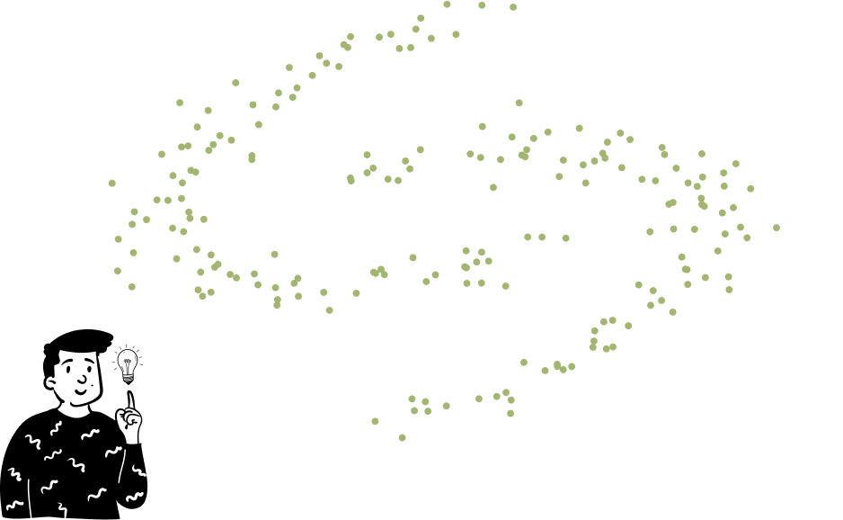
In these kinds of situations, the most common algorithms, such as SVD or PCA, don’t work very well. This is because they are based on the hypothesis that the space is Euclidean (linear). For example, imagine representing points that lie on a sphere by projecting them onto a plane. This would create a lot of noise that might distort the patterns originally present.
To reduce the dimensionality of these kinds of datasets, there are several options, but one of the most promising is the SOM. Indeed, all we need to use it is the dataset and a couple of parameters that we have to choose.
The SOM algorithm
In simple terms, what SOM does is perform an iterative sequence of training phases. At each epoch, the algorithm’s goal is to self-organize in order to best approximate the multidimensional space. To do this, it approximates the input dataset with many multidimensional vectors called codebooks. Having the same dimension as the points in the dataset, these codebooks create a set of reference points that represent the general tendency of the data. The objective now is to define how these codebooks are generated and where to place them in a 2-dimensional map.
Set-up
There are three main parameters that must be chosen before starting the algorithm. A key feature of the SOM is that the first of these three parameters deeply influences the result, while the other two have their pros and cons but don’t significantly alter the outcome.
Map shape
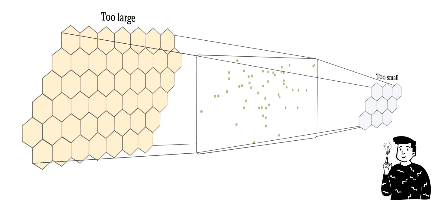
For each map, we must choose the number of codebooks for the base and the height to produce a rectangle composed of many cells, corresponding to the number of codebooks chosen. Unfortunately, there is no golden rule for choosing the right dimensions, but it is important to keep in mind that creating a map that is too large will lead to overfitting (remember that this algorithm can be used either as a density estimator or as a classifier), while a map that is too small tends to cluster the observations too much.
Cell shape
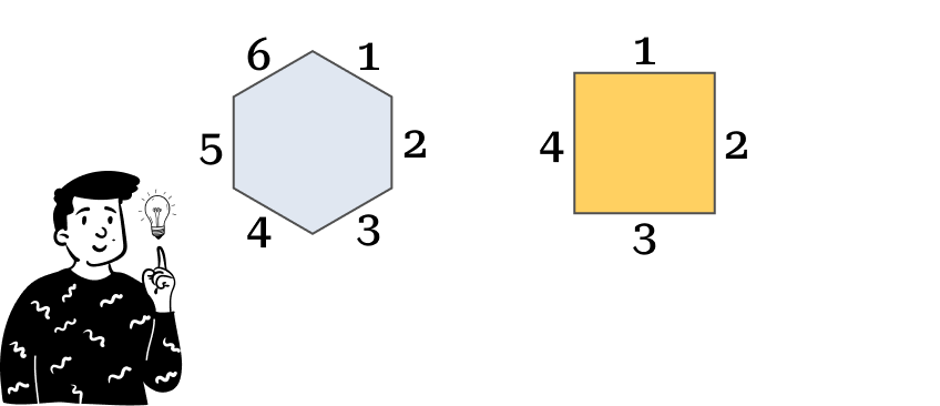
Each codebook is associated with a cell in the map, meaning that the map is the sum of many connected cells. One thing we can choose is the shape of these cells. There are plenty of options, but the most commonly used are:
Hexagonal shape
Square shape
Apparently, this choice might seem merely graphical, but as we’ll see later, the number of neighbors depends on the number of the cell’s sides.
Topology
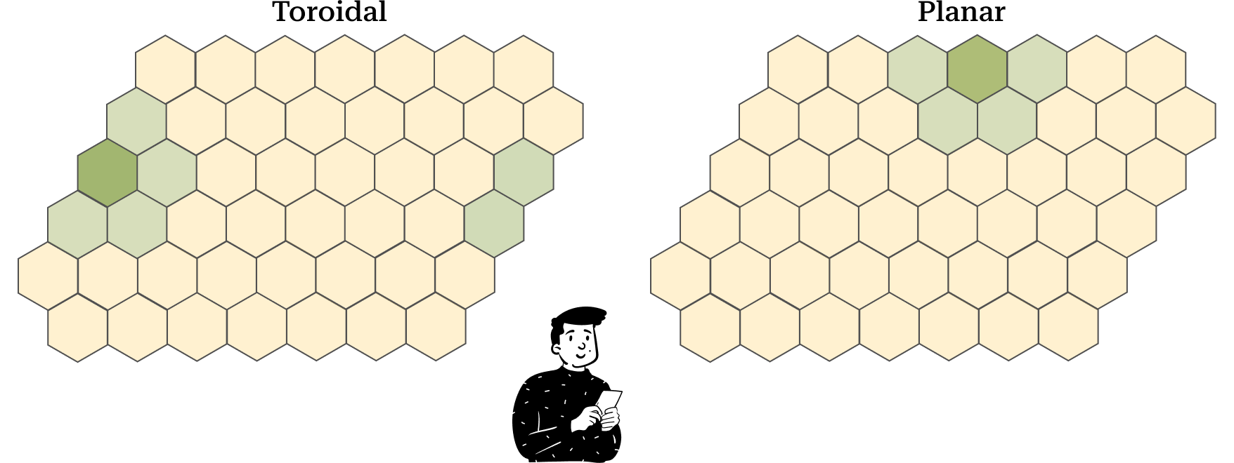
The last parameter we have to choose is the topology of the map. This term refers to the map's construction. One observation that might come to mind is that the cells at the border have fewer neighbors. To resolve this problem, we can define the map as a toroid. This way, we can eliminate the border effect present if we choose a planar map.
In the toroidal map, during the training phase, the surface wraps to form a toroid. By doing so, each cell has an equal number of neighbors. However, in the visualization process, the toroid reverts to a plane, and the cells at the extremes are connected with the cells on the opposite edge.
In the planar map, interpretation is easier, but the border effect problem emerges.
Initialization
Before starting the training process, it is necessary to assign an initial value to each codebook. There are two ways to do this:
Generate n multidimensional vectors randomly.
Sample n rows (vectors) from the dataset.
It can be proven that regardless of the option chosen, the algorithm arrives at the same result; the only difference is the rotation of the map.
Training
The training phase is very similar to that in K-NN. Indeed, in this case, we are dealing with unsupervised learning where each codebook competes with the others to adapt to the data (that’s why this kind of training is called competitive learning).
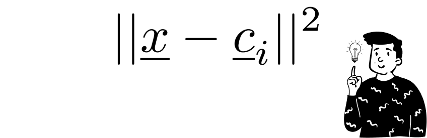
After initialization, each observation in the dataset is compared one at a time with the codebooks in the current epoch. For each codebook, the Euclidean distance between itself and the current observation is calculated.
After the initialization, each observation in the dataset is confronted one at the time with the codebooks at the current epoch. For each codebook it is calculated the euclidean distance between itself and the current observation.

The codebook that minimizes the distance becomes the Best Matching Unit (BMU) for the current observation.
Then, the BMU's values are updated to approximate the current observation. The updating expression is:

As you can see, the updating process is weighted by a function hh that we’ll discuss later. What you need to know is that as epochs progress, the influence of this function diminishes.
Along with the BMU, all other codebooks are updated using the same law, with the only difference being that the argument of the weighting function also includes the distance between the current codebook and the BMU:

This is the most important feature that this algorithm provides. It doesn’t just update the nearest codebook but the entire map. Obviously, the intensity of the update is lower for the codebooks that are farther away.


These three steps are repeated for each observation in the dataset. Once done, the algorithm has completed its first training epoch. Usually, the number of epochs is in the hundreds, but fortunately, the algorithm can stop early once the codebooks’ values converge between epochs.
Weighing function
The function h is the only dynamic element of the entire algorithm. It depends on two different arguments:
The current epoch.
The distance between the codebook and the current BMU.
Usually, the chosen function is the Gaussian kernel with a scaling factor:
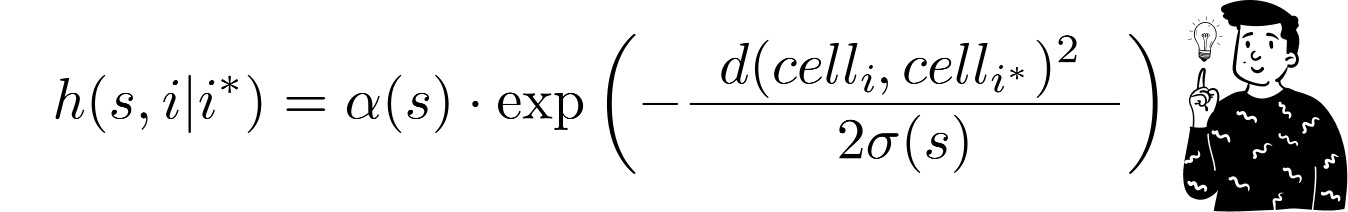
Where:
d is the Euclidean distance between the two codebooks.
σ(t) and α(t) are two monotone decreasing functions that act as intensity regulators. They both depend on the epoch’s value. Indeed, the function hh tends to shrink and flatten with each iteration.
The decrease in intensity is crucial for the correct execution of the algorithm. If it didn’t happen, each epoch could erase all the information learned up to that point.
SOM visualization
After the training process, it is possible to visualize the tuned codebooks. The best way to do this is by using component planes.
Component planes are maps that are characterized by coloring each cell based on the values assumed by the i-th component of the vector. By doing so, we can create one map for each dimension in the input dataset.
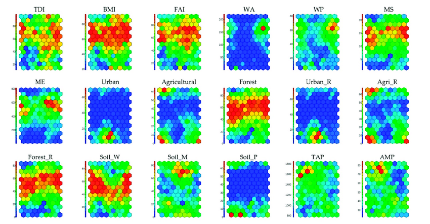
In cases where the input space has a relatively small dimension (4-5 dimensions), we can combine different component planes to see the complete trend.
To add more context to each map, one thing we can do is to overlay the observations on the map. This way, we can identify the most crowded cells.
Every time we see a SOM map, we must keep in mind that distances are not preserved. This means that cells near each other do not necessarily imply that their vectors are similar. Indeed, it is possible to find some cells that are empty of observations; their purpose is to create a kind of bridge between two zones in the input space. So, keep in mind that the space we see is continuous but also stretched.
Map quality
To measure the map quality, we can use two different metrics, both of which are averages of certain quantities:
Quantization Error: This shows how well the map adapts to the data. To calculate it, we simply average the Euclidean distances between the input data and their Best Matching Units.
Topographic Error: This helps to assess how much the map distorts the input space. To calculate it, we average the distances between neighboring codebooks. A small value indicates a small distortion.
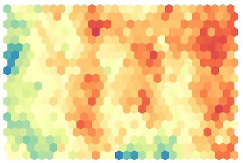
Voronoi tessellation
In the context of Self-Organizing Maps, Voronoi tessellation provides a useful way to visualize how the input space is partitioned among the neurons in the map. Each neuron can be considered a reference point, and its corresponding Voronoi cell includes all the input data points that are closer to it than to any other neuron. As the SOM algorithm progresses, neurons adjust their weights to better represent clusters in the data, effectively reshaping their Voronoi cells to align with the underlying data distribution.
This visualization helps in understanding how SOM preserves the topological properties of the input space. Indeed, the SOM:
Uses the input space to determine the BMU.
Uses a 2-dimensional space to determine how information is diffused among the cells of the map.