

From Pixels to Patterns: A Deep Dive into Convolutional Neural Networks
Episode 6 - CNNs is the core technology used for detecting more complex patterns inside audio, video and photos.

What CNNs are
Until this episode, all examples of neural networks I’ve provided were about fully connected ones. In simple terms, each neuron in these networks is connected to the neurons in the subsequent layer. However, the world of AI offers a wide variety of neural network structures, each with its own advantages and disadvantages. One such structure is the Convolutional Neural Network (CNN).

This type of network differs from the simpler fully connected ones because it contains one or more convolutional layers, which are well-suited to analyzing structured grid-like data. CNNs are widely used in computer vision for tasks such as image classification, object detection, and facial recognition, but they are also applicable to higher and lower-dimensional data structures like video and speech recognition.
Much like other types of neural networks, CNNs resemble processes occurring within the human body. Take, for example, the human visual cortex. As you read this post, your eyes capture images, and studies have shown that these images are passed through multiple levels of the visual cortex, each extracting particular features to help you better understand what you're seeing. CNNs (in the case of image recognition) work similarly, breaking down images into smaller sections and learning features hierarchically—from simple patterns like edges to complex objects.
Understanding Convolutions
As the name suggests, the convolution operation is central to CNNs. While this topic can quickly become overwhelming, I’ll provide a high-level explanation, focusing primarily on computer vision.
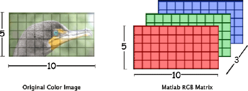
When you view an image (let’s assume it's grayscale for simplicity, I’ll talk about RGB images later), what you see is not what a computer sees. Instead, a grayscale image is represented as a matrix of numbers ranging from 0 (black) to 255 (white), with all the shades of gray in between.

This matrix serves as the input to the convolutional network, and since images have both height and width, this data is considered two-dimensional. This is why in the first diagram, you saw three rectangles representing the matrices fed into the network.
This concept applies to RGB images as well. In this case, instead of having a single grayscale channel, you have three channels—Red, Green, and Blue. By stacking these matrices, one on top of the other, you form a color image. In mathematical terms, this multidimensional matrix is called a tensor.
For simplicity’s sake, let’s stick with the grayscale example, using just one channel. The CNN’s goal is to learn complex patterns, and it does so in a commonsense way—by analyzing more than one pixel at a time. To identify whether a specific area of a photo represents, for example, a line, it’s clear you need to focus on more than just a single pixel.
Kernel matrix
This is where convolution comes in. The convolution operation merges two sets of information to produce a new meaningful representation. Inside the network, convolution is applied using a matrix called the Kernel, which acts as a filter. The Kernel is a smaller matrix, containing trainable weights, that is multiplied element-wise with the input matrix.

Each cell in the feature map is produced by multiplying the Kernel matrix with the input matrix, but the size of the feature map depends on two hyperparameters:
The sliding window: This refers to how the Kernel moves across the input image. By default, the boundaries of the Kernel align with the input image, but you can widen or narrow these boundaries by padding the input matrix with zeros or by modifying how the Kernel scans the image.
The stride: This indicates how far the Kernel moves at each step. If the stride is set to 1, the Kernel moves one pixel at a time. A larger stride results in a smaller feature map.
In summary, the Kernel synthesizes the input data. You can use multiple Kernels in each convolutional layer, and each one will extract different patterns from the image.
Shared weights
The values inside the Kernel are weights—no different from the weights in a simple neural network. These weights are optimized and used to perform linear combinations with the input matrix. The key difference is that the weights inside the Kernel are shared across all inputs in the layer.

Why is this? Imagine comparing two images of the number 7. You can recognize the number in each image, even though it may appear in different positions. The Kernel’s job is to identify patterns, so it needs to scan the entire image. By sharing weights, the network can recognize patterns regardless of where they appear within the image.
The Elements that Compose a CNN
Now that we’ve discussed convolution, let’s explore the architecture of a CNN. To understand the diagrams, there are two additional elements to introduce:
The pooling layer
The flattening operation
I promise these concepts are much simpler than convolutions.
Pooling layer
Using convolution increases the number of elements in the network, enriching the information at each layer. A pooling layer helps reduce the spatial dimensions of the data, shrinking each matrix within the tensor by reducing its height and width. This is done for several reasons:
Decreasing computational power
Reducing the number of parameters
Preventing overfitting
Extracting dominant features while discarding irrelevant information
There are various types of pooling layers, the most common being:
1. Max pooling
This takes the maximum value from a defined region of the tensor (usually feature maps). A larger region results in a smaller output matrix.
2. Average pooling
As the name suggests, this reduces the dimensions by averaging the values within a defined region of the feature map.

Flattering operation
After a series of convolutional and pooling layers, many tasks require a simple dense layer (as seen in previous episodes). To transition from a tensor to a vector, we use the flattening operation. This step concatenates all the values from the feature maps into a single long vector, with the size being the number of rows times the number of columns times the number of matrices.
Convolutional layer
As mentioned earlier, the convolutional layer consists of a Kernel matrix that extracts features from an image. Each layer can have multiple filter matrices, increasing the tensor’s dimensionality. After each convolutional operation, a bias is added to the feature map, followed by the activation function (commonly ReLU).

Putting all together
Now, let's step through the process illustrated in the first diagram:
First max-pooling

At this stage, the input tensor consists of 3 matrices, each of size 128x128 (e.g., an RGB image). The first operation is max pooling, which reduces the size of the image to decrease the number of parameters. In this case, the image size is halved, likely using a pooling window of 2x2 with a stride of 2.

First convolution
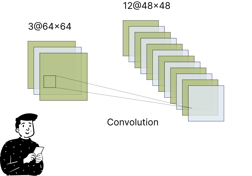
The "shrunken" image is now used by the network to learn patterns. In this example, 12 different Kernel filters are applied to capture various patterns. Due to padding and stride, the output has a different size than the input.
Second max-pooling
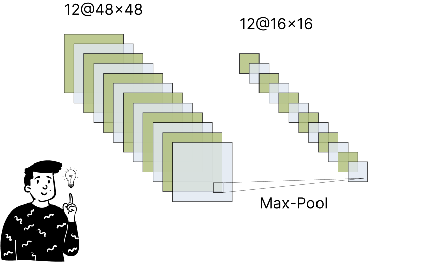
This step is similar to the first max-pooling layer. The feature maps are further reduced, and this operation often follows a convolutional layer, especially before a fully connected dense layer.
Flattering

Finally, the tensor is converted into a vector. As previously discussed, the tensor’s elements are concatenated into a vector with 12x16x16=3,072 units, which is then fed into a dense layer with 64 output neurons.
This CNN architecture is one of the most fundamental in the world of neural networks. Of course, it is not the only type and is rarely used alone. In the next episode, we’ll explore Recurrent Neural Networks (RNNs), which are designed to remember previous inputs over time.
(Probably if you click on my account you can already see the next episode)