

The Fundamentals of Decision Tree Learning
Understanding the mechanics, optimization, and practical applications of decision trees in machine learning.

The decision tree is a very popular algorithm used for both classification and regression tasks, especially when interpretability is a key concern. It also serves as the foundation for many more complex algorithms, such as Random Forest and Gradient Boosting.
We can think of this model as a sequence of boolean questions, where at each stage, the classifier select the "question” that best discriminate the dataset with respect to the target variable Y.
In this post I will cover the core theory and essential concepts of this model. To do so we’ll explore:
How a decision tree is constructed
Its main components
The different types of splits
How classification works
The concept of impurity
Gini split
How it handle quantitative targets
The stopping rule
Pre-pruning
Post-pruning
Decision tree learning
As mentioned earlier this classifier is highly popular due to its straightforward interpretability. Unlike other models that require complex plots, a decision tree can be graphically represented using a simple diagram that illustrates the splits made at each node.
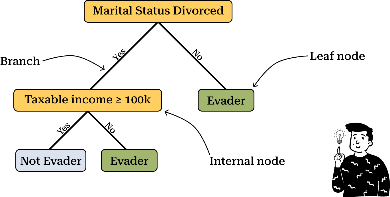
In the diagram above there are three key elements to consider:
Internal Node: Represents the question used to split the dataset into two parts. The goal is to determine the best split, which involves selecting the appropriate variable and deciding on the optimal threshold value.
Branch: Represents the connection between two nodes. In most cases, each split results in two branches, corresponding to a dichotomous decision, such as "Yes" or "No."
Leaf Node: The final node in the tree, used to classify an observation into a specific category.
Now let's consider an example. Suppose we have a new individual who is divorced and has a taxable income below $100K. To determine whether this person is an evader, we follow the path dictated by the tree. Starting from the root node, we take the "Yes" branch, leading us to another internal node. Based on the individual’s characteristics, we then follow the "No" branch, classifying the observation as an evader.
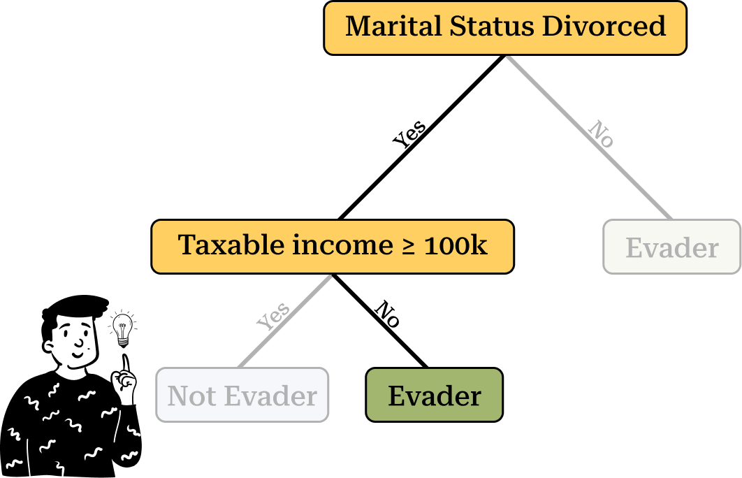
It is important to note that if the individual were not divorced, they would always be classified as an evader, regardless of their taxable income.
Different Types of Splits
Before using a decision tree we must define the number of splits at each node. The best practice is to use a binary split, where the dataset is divided into two subsets at each step.
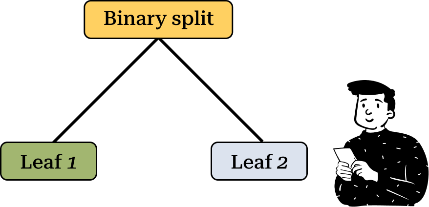
This type of split is the default in Classification and Regression Trees (CART), which is one of the most widely used decision tree algorithms in machine learning. CART supports both qualitative and quantitative targets, making it highly versatile. The decision tree implementation in sklearn is based on CART, so we will also follow this approach.
If you need to apply a decision tree to a dataset it is advisable to transform ordinal variables into nominal ones. This is because a continuous or ordinal variable with n modalities can create up to n-1 possible splits. In contrast, a nominal variable allows for a maximum of 2ⁿ⁻¹ - 1 admissible splits.
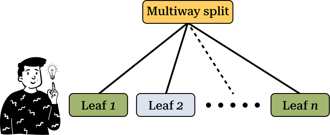
On the other hand, multi-way splits divide the dataset into multiple groups at each node. However, this approach is less commonly used because generating too many sub-groups results in nodes with too few observations, increasing the risk of overfitting.
Classification with Majority Vote
Each leaf node assigns a class label to observations that reach it. One of the main objectives of training a decision tree is to correctly classify new data. The most common method for classification is majority voting.
This technique is widely used in other machine learning algorithms, such as k-NN. The assumption is straightforward: the class with the highest number of training observations in a node is the predicted class. In the case of a binary target, the ideal scenario is having each leaf contain only one class. However, in practice, leaf nodes often contain instances from both classes. Therefore, we compute the proportion of observations belonging to each class (e.g., Y=1 and Y=0), and this proportion represents the probability of belonging to a specific class at that node.
Thus, for each leaf, we not only determine the most probable class but also assign an associated probability. This probability is crucial in machine learning, as many performance metrics rely on it.
How to Determine the Optimal Split
A key aspect of decision tree algorithms is defining the optimal split at each node. To do so, we use a metric that evaluates the best possible split based on both the predictor and the target variable. Ideally the child nodes should be more homogeneous than their parent node. This concept is closely tied to the idea of impurity, and in the CART algorithm, we choose the split that results in the highest impurity decrease between the parent node and its children.
Gini’s split
For categorical targets (e.g., a binary classification problem), the most commonly used impurity metric is the Gini index, defined as:

Where f is the proportion of elements that belongs to the class j-th at the node t.
The Gini index has a maximum value when all classes are equally represented in a node, and a minimum value when the node contains only one class. The ideal condition in a decision tree is to minimize the Gini index at each split, ensuring that the resulting leaves classify observations with high certainty.
To choose the best split, decision trees compute the Gini split metric:
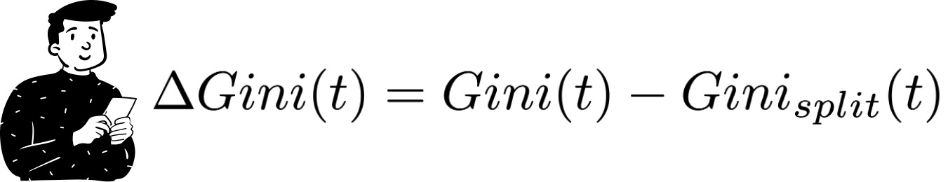
This metric measures the difference between the Gini index of the root node and the weighted sum of the Gini indices of its children. The weights are calculated based on the proportion of observations that pass through each child’s node. The objective is to select the split that maximizes the Gini index.
Splitting for Quantitative Targets
The Gini index applies only to classification problems. For regression trees a different approach is needed. In the CART framework the key metric is variance.
A good split minimizes the variance within each node while maximizing the variance between nodes. This means that, for each possible split, the algorithm computes the weighted sum of variances in the child nodes and selects the split that minimizes this value.
There are many alternative impurity metrics, including cross-entropy, Chi-square, and R-square, but they all follow the same fundamental principle: maximizing homogeneity within nodes and heterogeneity between nodes.
The stopping rule
Before running a decision tree algorithm, it is crucial to define a stopping rule—a criterion that determines when the tree should stop growing. Without such a rule, the tree could continue splitting until each observation has its own leaf, resulting in overfitting.
To control model complexity, stopping rules are applied in two phases:
Pre-pruning: Before training, we set constraints such as the maximum number of nodes or the minimum number of observations per node.
Post-pruning: After training, we remove nodes that contribute to overfitting. This is done using cross-validation to determine the optimal number of nodes that minimize a performance metric.
There are several post-pruning techniques. One common method involves using a complexity parameter, similar to the regularization term in Lasso regression. In this case, the penalty is applied to the performance metric, reducing the risk of overfitting.