


As promised in this last episode of the short series about Bayesian statistics, I will talk about a very famous method used to sample from a probability distribution: the Markov Chain Monte Carlo (MCMC). The goal is to produce a sequence of values that are governed by some probability distribution.
One thing you might ask is why we need to approximate the sampling if we have the function that governs events. This question is not so trivial. Indeed, when we work in the frequentist realm, most of the time the theorem of the central limit helps us by allowing the use of the Normal distribution if we want to make inferences on a large set of variables that are independent and identically distributed (IID).
But in a dynamic environment such as Bayesian statistics the identical distribution of the parameter that governs values (by definition) changes over time. Another problem is that when we use a continuous variable to derive the denominator used in Bayes' theorem, we have to resolve an integral that might not be so trivial.
For these reasons, in many fields, MCMC methods are widely used because they can make good approximations (thanks to their properties) and don’t require too much computational power.
Monte Carlo approximation
The key concepts that are merged together in MCMC are the Monte Carlo approximation and the Markov Chain. Although this approximation is used only after the sampling process has been made by creating a chain, it is better to start with it because it can help us understand why we also need a chain to resolve integrals.
The idea can be used to derive every expected value we want. Indeed, the theory underlying it is pretty simple. The “only” constraint is that the variable has to be IID, but if it is so, we can apply the law of large numbers, which in practice states:
Given a set of n samples, if the number n goes to infinity, the probability that the sample mean equals the population mean is 1.
Using this theorem helps us derive the expected value of any given distribution by using a sufficiently large sample:
The Monte Carlo Method can also be used to derive the expected value of the posterior distribution. To do that, there are various ways. If we are able to use the posterior distribution, we just need to sample a sufficiently large number of values from the distribution and then calculate the sample mean.
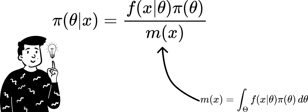
Approximate the Bayes theorem
Thanks to calculus rules, we can separate the constant elements inside an integral to simplify it.
In this way, we can apply the Monte Carlo principle to both the numerator and the denominator. This step is pretty tedious. Indeed, we have to remember that probability distributions are functions, such as log(x). This means that by giving a value as input, we can get a value as output. So, to approximate the numerator (and the denominator), we can treat one of the probability distributions as a normal function and the other as the distribution from which we sample. Because the likelihood function f(x|θ) requires the value of θ as input, we’ll use the prior distribution of θ for both integrals to sample from.
Python example
What we’re going to do now is a Python simulation that shows what this algorithm requires. If you want you can find all the code used in this post in my GitHub repository. Here I show you just the key aspects.
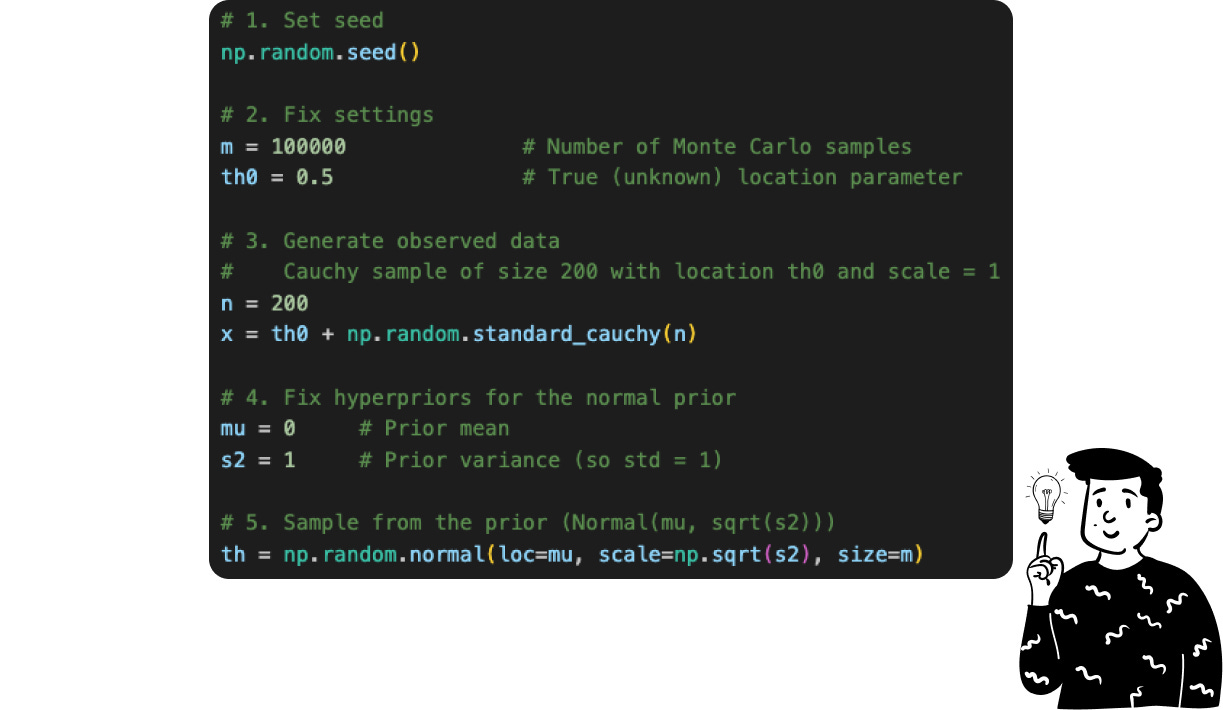
Suppose that we don’t know that the posterior distribution of our data follows a Cauchy distribution with parameter θ equal to 0.5, and we want to derive it using the Monte Carlo approximation.
The first thing to do is to define the parameters, which are essential for the simulation and approximation process. These parameters include:
th0(True Parameter): Represents the true value of the parameter we aim to estimate. In practical scenarios, this value is unknown and estimated from data.m(Number of Monte Carlo Samples): Determines the number of samples drawn from the prior distribution to approximate the posterior distribution.n(Number of Observed Data Points): Specifies the number of data points to generate from the Cauchy distribution.muands2(prior hyperparameters): They are known since belongs to the prior distribution, that in this case is the normal standard

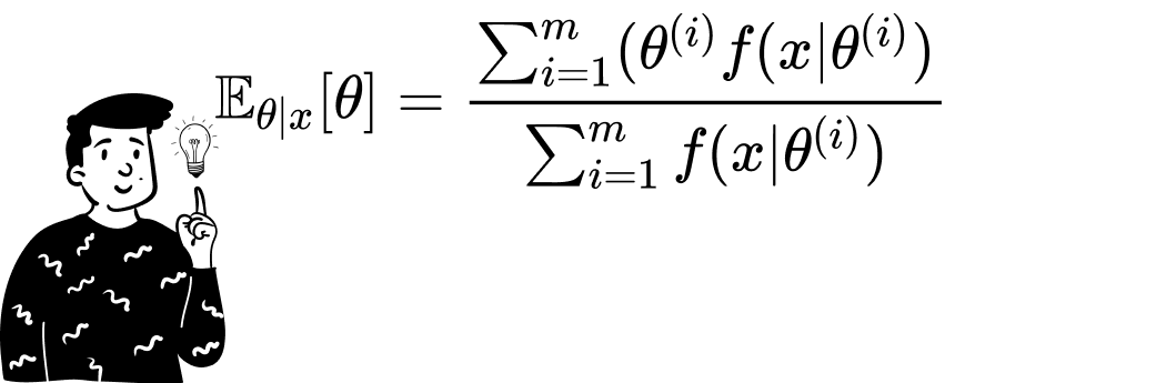
Once we have the sample containing the m values of θ, we can calculate the expected value of the posterior distribution by simply taking the sample mean. This is the average of the m outputs produced by the function θ • f(x|θ). To facilitate the arithmetic operations, I have used the log-likelihood instead of the likelihood since the product of elements becomes the sum of the log elements.
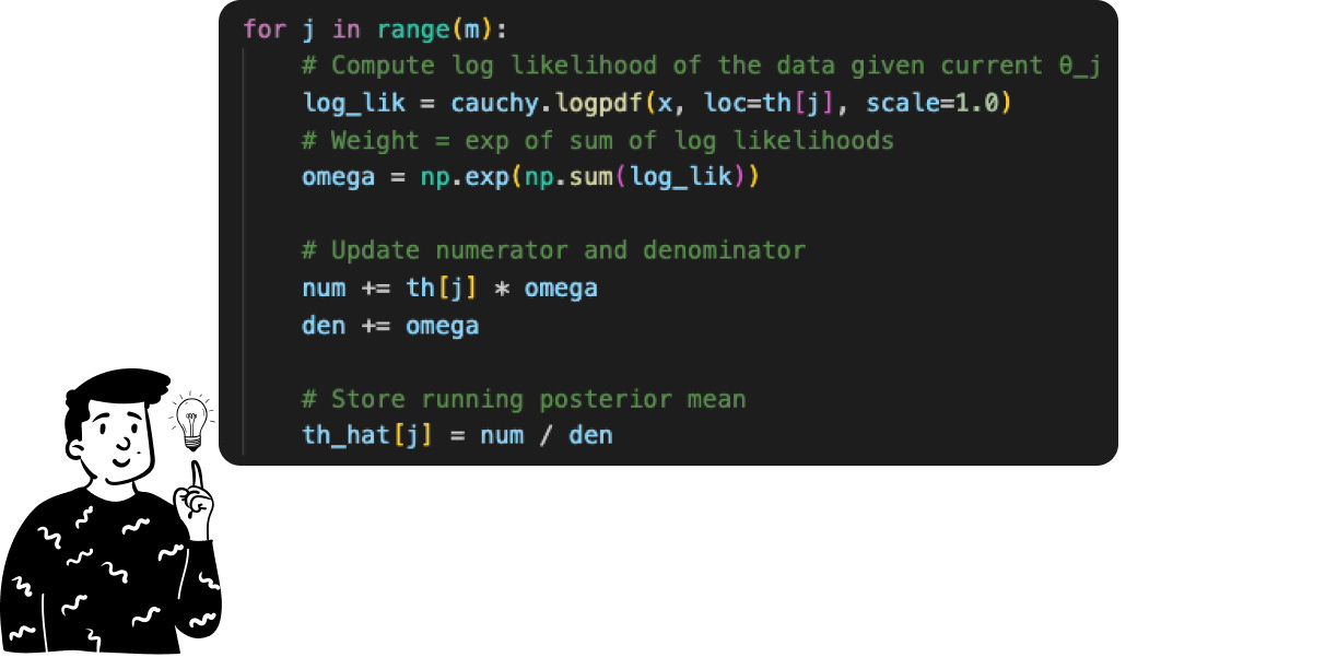
By doing so, we have just made the Monte Carlo approximation, which can lead to very promising results.
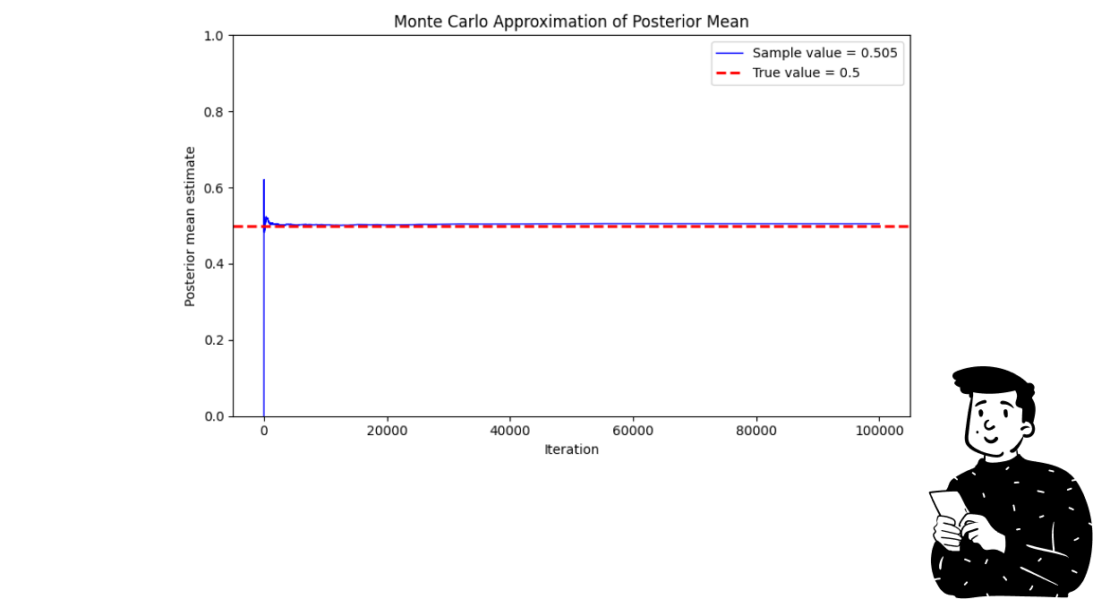
The plot above shows how the Monte Carlo algorithm approximates the real parameter at each iteration. What you can see is that in the initial steps, the blue line (which refers to the sample value) produces some fluctuations. This is caused by the fact that it is a stochastic process, and at each iteration, the influence of one point tends to decrease. That’s why it is very probable to see strong fluctuations in the first steps.
Monte Carlo Markov Chain
What you might have noticed from the Monte Carlo Method is that it doesn’t resolve the problem of approximating the sampling function. Indeed, in order to estimate the posterior mean, you have already accomplished the sample. To tackle this problem, we use Markov Chain Monte Carlo. Its idea is to create a chain of values for θ that, as the number of steps increases, the chain converges to the approximating distribution.
This family of algorithms is characterized by respecting the ergodic property. This means that whatever value we choose to start the chain with can sample the entire space. Thanks to this property, the algorithm guarantees that, for whatever starting value we choose, at some point, the extracted values will resemble those we sample from the approximating distribution.
There are many algorithms that belong to this family. The most famous are the Gibbs Sampler, the Metropolis-Hastings, and the Random Walk Metropolis-Hastings. In this post, we’ll focus on the latter.
Random Walk Metropolis-Hastings
Continuing our exploration of MCMC methods in Bayesian statistics, let's delve into the Random Walk Metropolis-Hastings (RWMH) algorithm. RWMH is a fundamental technique for sampling from complex probability distributions, especially when direct sampling is infeasible. The essence of RWMH lies in constructing a Markov chain that eventually mirrors the target distribution, allowing us to approximate it through the generated samples.
At its core, RWMH operates by initiating the chain with a starting value θ₀, and iteratively proposing new candidate states θ′, by adding a random perturbation to the current state θₜ. This perturbation is typically drawn from a symmetric distribution, such as a Gaussian , ensuring that the proposal mechanism does not favor any direction in the parameter space.
Once a candidate θ′ is proposed, the algorithm assesses its suitability relative to the target distribution p(θ). This assessment is quantified through an acceptance ratio:
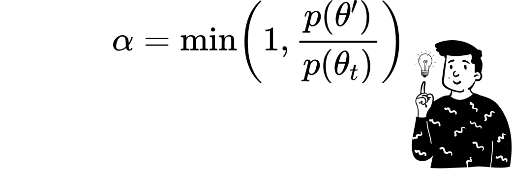
Given the symmetry of the proposal distribution, the ratio of proposal probabilities cancels out, simplifying the acceptance criterion. A uniform random number u drawn from the interval [0,1] determines whether the candidate is accepted. If u≤α, the proposal θ′ becomes the next state θₜ₊₁; otherwise, the chain remains at θₜ.
This mechanism ensures that the chain spends more time in regions of higher probability density, effectively capturing the characteristics of the target distribution over time. However, the efficiency of RWMH hinges on the choice of the step size σ. A step size that's too small leads to slow exploration and high autocorrelation between samples, while one that's too large results in frequent rejections, hindering the chain's ability to explore the parameter space adequately. Striking the right balance is crucial for the algorithm's performance.
Moreover, the initial iterations of the chain, often referred to as the "burn-in" period, may not represent the target distribution well. Discarding these early samples allows the chain to stabilize and better reflect the underlying distribution. Even after convergence, successive samples may exhibit autocorrelation, meaning that each sample is not entirely independent of the previous ones. Techniques such as thinning, where only every k-th sample is retained, can help mitigate this issue, though it reduces the effective sample size.
Python example
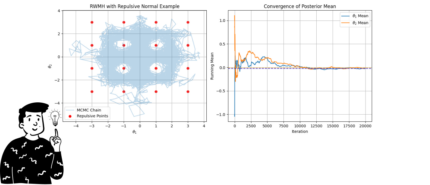
In this specific example, we’ll use the RWMH to sample from the repulsive normal distribution. You can think of it as a multivariate normal distribution that has some points (in this example, 16) with a probability almost equal to 0. As you can imagine, sampling from such a distribution is very difficult. For this reason, we’ll use a Markov chain.
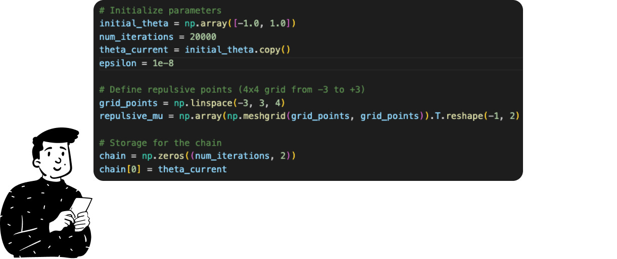
As in the previous example, we start by setting the hyperparameters:
The initial position in the space where the random walk starts.
The number of iterations.
The number of repulsive points and their coordinates.
An arbitrary parameter to avoid division by zero (the epsilon variable).
The whole MCMC sampling in Python takes just 6 lines of code, and the core element is the
ifstatement inside it that represents the acceptance rule. Since, for the same reason as the previous example, I have used the log transformation, the acceptance ratio is just a difference between the current posterior and the proposed posterior.
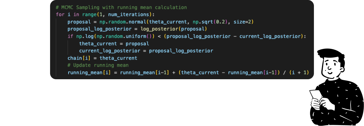
Here, we can both produce a sample set with a specific chain and calculate the summary (average) using the Monte Carlo approximation.
I hope you’ve enjoyed this brief series about Bayesian statistics. This is also the last post of 2024, so Happy New Year to everyone! We’ll see next year with many new posts, starting with LSTM and SOM.