


Continuing with the series of dimensionality reduction algorithms, one noteworthy procedure is random projections.
Most of the time in statistics, when we design an algorithm that inevitably causes some loss of information, we choose a cost function that globally represents the error resulting from the applied method. The goal is to tune the algorithm to minimize the loss of information globally. This is the approach used by algorithms such as SOM and NMF.
A Comprehensive Guide to Self-Organizing Maps (Kohonen Networks) for Dimensionality Reduction

The Self-Organizing Maps (also known as Kohonen maps, named after their inventor Teuvo Kohonen) are a fundamental neural network algorithm. Although their initial goal was different, this unsupervised machine learning technique has gained importance in dimensionality reduction applications, especially when dealing with multidimensional datasets where po…
However, random projection takes a completely different approach. Instead of simplifying high-dimensional datasets based on a rule that optimizes a global function, it focuses on each individual observation, providing a representation that distorts them by a fixed amount.
In this post we’ll cover:
Why a global approximation isn’t always the best choice
How to measure and control distortion
How to find the best space to represent data (Johnson-Lindenstrauss Lemma)
How random projections work in practice
What their properties are
A Python snippet
So, let’s dive in.
What Local Preservation Means
Since, as we’ll see later, random projections are a technique well-suited for high-dimensional data (in the thousands of dimensions), I’ll first demonstrate the key distinction between optimizing a global function versus many local functions that focus on each observation, using regression as an example.
Trying to represent the relationship between two variables by assuming that all observations lie on a straight line is a bold assumption. In reality, outcomes often depend significantly on randomness. Even when the correlation (dependence) between variables is strong, noise causes some loss of information when approximating the trend using a straight line.
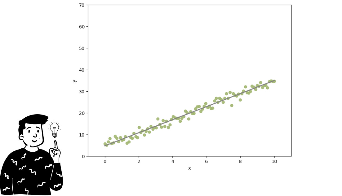
To approximate the data in the best possible way, we use a technique called Ordinary Least Squares (OLS). Its goal is to minimize the average error produced by the approximating function (in this case, the gray line) across all points simultaneously. As long as the data generally follows the same trend, this method works well. However, when we allow observations to exist in a space with thousands of dimensions, it is likely that no single trend works well for every point. Consider the plot below:
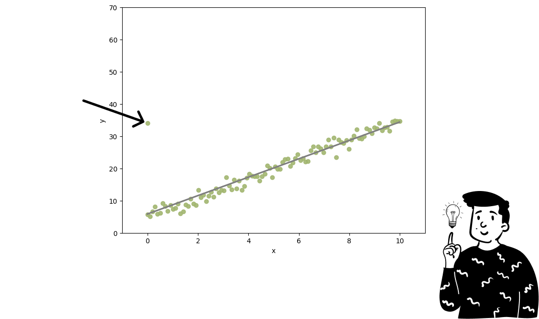
In this scenario OLS remains a reasonable choice (due to the low number of outliers and the scope of the analysis). However, isolated observations are poorly represented because their weights are too small to significantly influence the direction of the line.
Random projections aim to give more importance to each observation compared to dimensionality reduction algorithms that rely on global cost functions.
An important point to note is that while OLS is often understood as a method for regressing one variable on another, algebraically, it projects data onto a subspace, making it, in essence, a dimensionality reduction tool.
How to Measure Distortion
Whether using a global function or not, the core principle of fine-tuning tasks is to find something to optimize, which requires a way to measure it.
In random projections, distortion is measured as the difference in norms between the input data and the reduced data. For each observation, the norm must not exceed a fixed threshold T .

Why measure the difference in norms specifically? There are two main reasons:
Most algorithms in data science, such as K-NN, use Euclidean distance as a measure.
The Johnson-Lindenstrauss Lemma, which we’ll discuss next, relies on it.
Johnson-Lindenstrauss Lemma
In mathematics, a multidimensional function where the difference in norms of the images of two vectors has upper and lower bounds proportional to the difference in norms of the vectors themselves is called a limited distortion function. This is the function we aim to find with random projections to regress data onto its space.
Unfortunately, the existence of such a function isn’t guaranteed. However, the Johnson-Lindenstrauss Lemma states:
Given an approximating error 0<ε<1 and a number of elements n, there exists a limited distortion function in a space of the size:
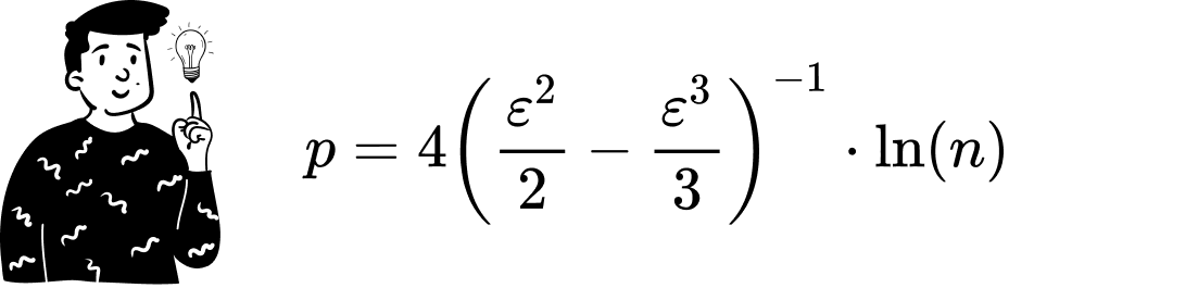
This lemma tells us that the optimal space for projecting data has p-dimensions. From the formula, we can observe:
he approximation error has a significant impact: smaller ε (due to the -1 in the numerator) increases p.
The number of points n to approximate also increases p, but logarithmically, which mitigates the impact.
The input space size isn’t a constraint, meaning p could sometimes exceed the input space.
To reduce the risk of p exceeding the input space, random projections are typically applied to enormous datasets, making this scenario highly unlikely.
How Random Projections Work
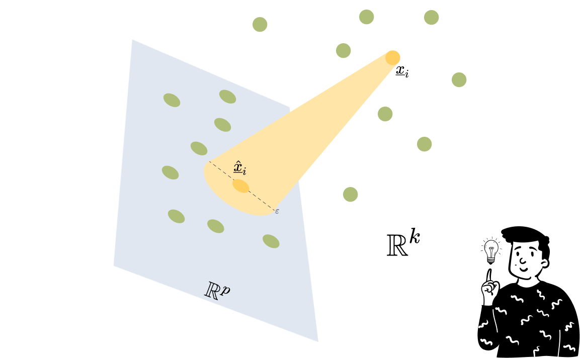
To create a limited distortion function in a p-dimensional subspace, random projection constructs a matrix R with as many rows as the input data and p columns. Each entry in R is a random variable independently and identically distributed according to a standard normal distribution. By multiplying the input data matrix by R:

The lemma guarantees that the resulting matrix has limited distortion with a probability of 1/n.
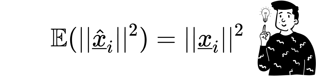
In theory the algorithm would generate multiple random matrices R until one satisfies the distortion property. However, this is computationally infeasible for large and dynamic datasets. Instead, we settle for the first random matrix R. Because its entries follow a normal distribution, the expected value of the squared norms of the approximated observations equals the squared norms of their original counterparts.
Other distributions can generate R , but the standard normal distribution is the most common, as it supports the proof of the lemma. For extremely large datasets (e.g., billions of images), an alternative distribution where P(X=-1)=P(X=1)=0.5 may be preferable
Probability of Distortion
The primary goal of random projections is to minimize distortion for each observation, and the expected value guarantees this. Additionally, using Markov’s inequality, we can calculate the probability of distortion for each observation:
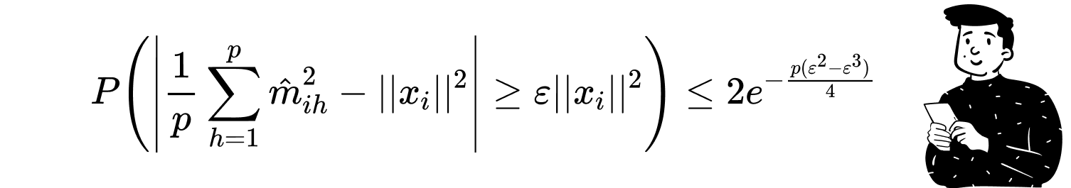
As the size of the projection space increases, the probability of distortion decreases. Conversely, a smaller approximation error increases the probability of distortion.
Python implementation
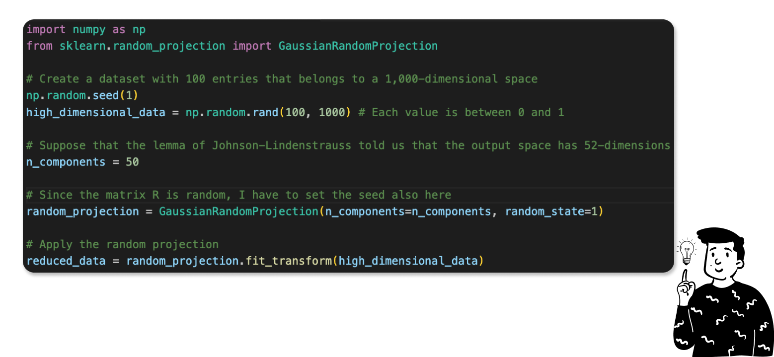
If you want to download the file, here is the link to my GitHub repository.
Random projections offer a potent alternative to conventional dimensionality reduction techniques by prioritizing local structures over minimizing global cost functions. This is achieved through randomness, which distorts individual observations within predetermined boundaries. Though counterintuitive compared to methods like PCA or NMF, random projections are efficient and scalable, making them indispensable for managing high-dimensional datasets. By leveraging the Johnson-Lindenstrauss Lemma, random projections strike a balance between simplicity, computational tractability, and accuracy, showcasing their utility in various applications.