

How to increase the performance of a classifier by using the dimensionality reduction tools
Exploring the Impact of Dimensionality Reduction on Decision Tree Performance for Human Activity Recognition

Currently, I’m writing my bachelor’s thesis in Statistics, focusing on the combination of dimensionality reduction techniques with ensemble algorithms. The first step in this process is gathering information from existing literature. One of the most interesting papers I found is Cann, Matthew. "Feature Reduction Using PCA, LDA, and PCA+LDA to Improve Decision Tree C4.5 Classification of Human Activity Recognition Dataset.” (2020).
My goal is to use this paper as a guideline to conduct my own analysis, implementing an autoencoder as well, to examine how different preprocessing techniques impact classifier performance in terms of accuracy (a symmetric measure) and F1-score (an asymmetric measure).
About the Paper
This paper introduces a new preprocessing step before applying a classification tree. The authors tested four different classifiers, each utilizing a different preprocessing technique:
Standardization only.
Standardization followed by PCA.
Standardization followed by LDA.
Standardization, PCA, and then LDA.
As you can see, every technique includes standardization. While not strictly necessary (only PCA requires it), standardization is commonly used because it enhances computational efficiency by ensuring that all variables have the same scale, reducing numerical instability.
The Fundamentals of Decision Tree Learning

The decision tree is a very popular algorithm used for both classification and regression tasks, especially when interpretability is a key concern. It also serves as the foundation for many more complex algorithms, such as Random Forest and Gradient Boosting.
In a previous post, we discussed decision trees, so I assume you are familiar with their strengths and weaknesses. One of their key advantages is their robustness to preprocessing; most decision tree-based algorithms do not require extensive preprocessing. However, if we were to choose a preprocessing technique, handling collinearity would be a priority. As the paper states:
The C4.5 [Decision tree] algorithm tends to overfit data that has many irrelevant features causing an increase in misclassification on testing sets.
About the Dataset
The dataset used to evaluate the preprocessing techniques was created by Reyes-Ortiz, J., Anguita, D., Ghio, A., Oneto, L., & Parra, X. (2013). Human Activity Recognition Using Smartphones [Dataset].
This dataset captures sensor readings from 30 volunteers (aged 19 to 48) performing six common activities: walking, walking upstairs, walking downstairs, sitting, standing, and lying down. Features were extracted from both the time and frequency domains.
Since we have six target classes, the maximum number of dimensions that LDA can reduce the feature space to is 6 - 1 = 5.
Another important aspect is the dataset's high-dimensional nature, with over 500 covariates. This makes it likely that some variables are highly correlated, leading to multicollinearity. The two common approaches to address this issue are:
Deleting some variables.
Reducing the feature space using techniques like PCA or LDA.
My Analysis
Now, let’s get into my analysis. This post does not include all the code, as it would be too lengthy. However, if you're interested, you can check my Kaggle notebook, where I provide the full implementation, including all libraries used.
Importing the Dataset
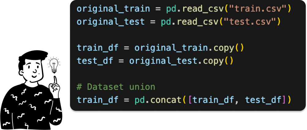
As a best practice, I first import the dataset and then work with a copy. In the code snippet provided in my notebook, I concatenate the training and test sets because the paper evaluates performance using 10-fold cross-validation. To clarify, cross-validation involves training the classifier 10 times, each time using 90% of the data for training and 10% for validation, with a different validation set in each fold.
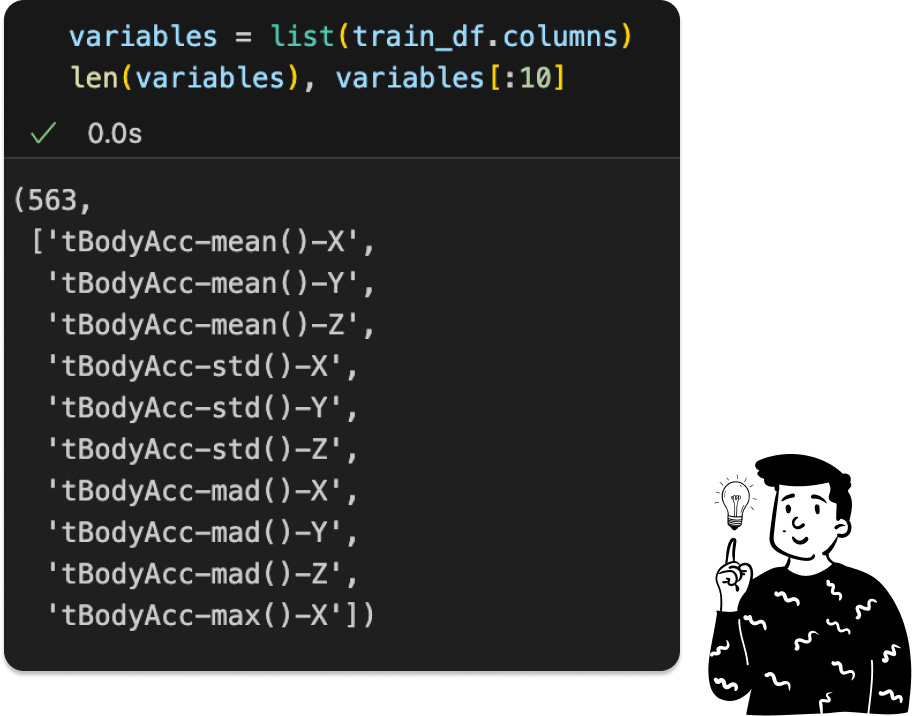
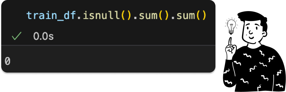
The dataset contains 563 features, posing a high risk of multicollinearity. Before addressing that, let's examine the target distribution.
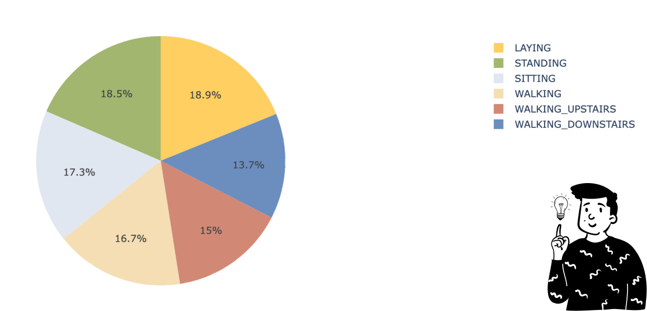
Fortunately, the dataset has a balanced distribution across classes, so no resampling is needed. Also, as the dataset description states, there are no missing values, eliminating the need for imputation.
Multicollinearity
To detect multicollinearity, we can't rely on a correlation matrix because a 562x562 matrix is impractical. Instead, we use the Variance Inflation Factor (VIF), which measures how much the variance of a predictor increases due to collinearity.
This metric is calculated by performing a linear regression of the residual of one variable against all the others. Then, we calculate the R² value to determine how much the variance of the variable exceeds the variance of the same variable if there were perfect correlation among the covariates. A higher R² value indicates a more significant problem with multicollinearity.
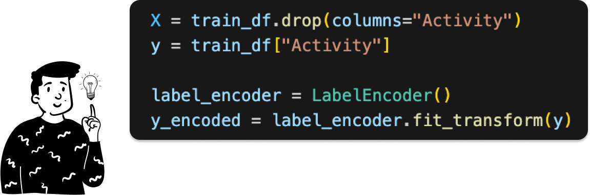
I first separate the target variable (Activity) from the covariates, then compute the VIF values.
At this point I have calculated the VIF:
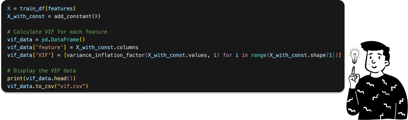
Since this computation is time-consuming (taking around 6 minutes), I save the results in a CSV file to avoid recalculating them each time.

Initial tests revealed extremely high VIF values for several variables. To make the results more interpretable, I applied a log transformation.
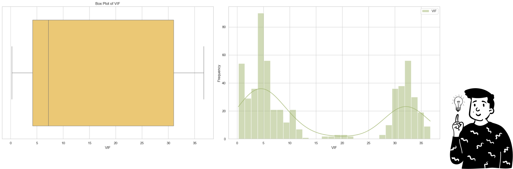
From the VIF distribution, we see two main clusters of variables. The median VIF value after log transformation is 7.27, which corresponds to an actual value of approximately e⁷𝄒⁷²=1,436. Typically, variables with VIF values above 4 are considered problematic, indicating a significant multicollinearity issue in this dataset.
Exploratory Data Analysis
Since this post focuses on preprocessing techniques, I won’t delve too deeply into exploratory data analysis if you want to learn more I suggest you to take a look at this notebook.
The only thing I’ve done so far is perform a t-SNE on the target variable. However, before showing you the results, I think it’s important to discuss some of the criticisms surrounding t-SNE and SNE in general. Although this non-linear dimensionality reduction technique is widely used, it has been proven that it can be quite unstable. This is because it attempts to preserve the original positions of points using a probability distribution instead of a distance metric. To determine the fit of a point in the chosen distribution, it uses a parameter called perplexity, which is quite common in information theory. This parameter helps us define how close points need to be to each other to be considered neighbors. However, the SNE is heavily influenced by this parameter, and there’s no clear way to derive it. Instead, we can only try different values empirically and see if the plots maintain the same structure.
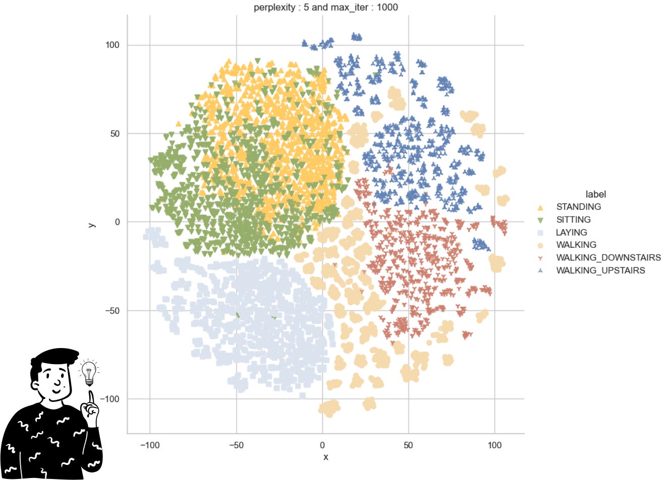
Looking at the t-SNE plot we observe:
The actions of being standing and being sitting are very similar to themselves; this suggests that the classifier will have some difficulties doing it.
The action of walking is the most variable since it is the most sparse across the plot.
Classification algorithms
The paper has used as a classification algorithm the decision tree, precisely the C4.5. Unfortunately, there isn’t a specific Python library for it, but we can use the DecisionTreeClassifier from Scikit-Learn and use the entropy criterion instead of Gini’s one.
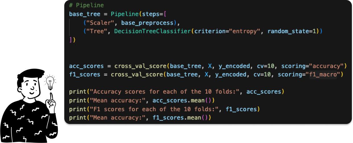
Base tree
Since with the PCA we’ll have to find some tuning parameters for all of the classifiers, I have decided to make a unique pipeline for each of them, and in shit case it is:

In practice, what it does is a simple standardization, and then all the features are passed to the decision tree to be used in order to fit the classifier.
At this point, we can calculate the cross-validated Accuracy and F1 Score. Before doing so, let’s clarify something. Since we have a multi-class target, all asymmetric metrics (like recall, precision, and F1) are not feasible. However, it’s possible to calculate the F1 score in different ways. One approach is using the f1_macro. This approach involves averaging the F1 score calculated for each modality, assuming it’s a binary classification problem. In this case, only the studied class is set to 1, while all other classes are set to Y=0. This approach makes all asymmetric metrics feasible. Alternatively, we could have used the f1_weighted, where the average is weighted by the number of each class. However, as shown in the pie chart, there’s no imbalance between the classes.
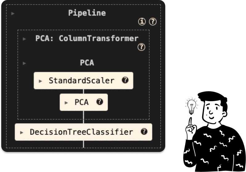
PCA tree
In this case, the pipeline consists of two preprocessing steps: standardization and PCA. The next step is to determine the optimal number of components to retain. Instead of relying solely on the cumulative explained variance, we’ll use the optimal number of components based on the accuracy of the classifier, as suggested in the original paper.
To be more specific, here is the code:
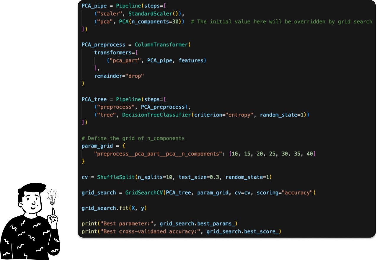
The original paper found the optimal number of components to be 30; in our case, the optimal number is 35. This divergence might be due to the fact that we’re using some libraries that are a bit different.
LDA tree
Here we can’t choose the optimal number of components since the LDA will produce at most 6-1 number of latent variables, where 6 in this case represents the number of modalities of the target, and since we’re passing from a dataset with 562 features to one that has only 5, we keep all of them, and the pipeline is defined as follows:
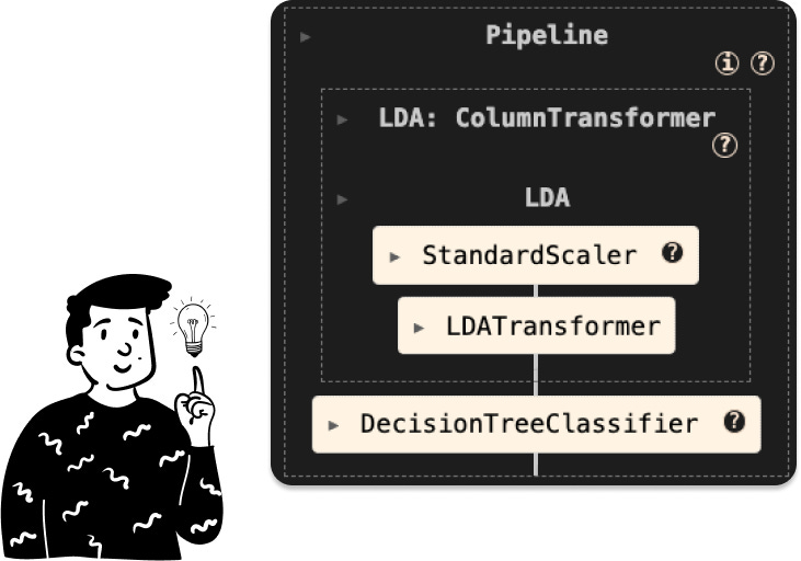
Where the LDATransformer is a custom class that I made for it:

Anyway, at the end of the post, I’ll show you the results, but before that, let’s introduce the last pre-processing technique that I have opted for.
Autoencoder tree
This technique is the only one among the four that doesn’t require a linear dimensionality reduction. In fact, an autoencoder is a specialized neural network that accepts a vector of k dimensions as input and produces a vector of q dimensions (with q typically being less than k) that effectively captures the essential features of the input space.
As in the LDA case, even here I have created a specific class in order to create a pipeline for the decision tree.

So the pipeline to train such a classifier is the following:
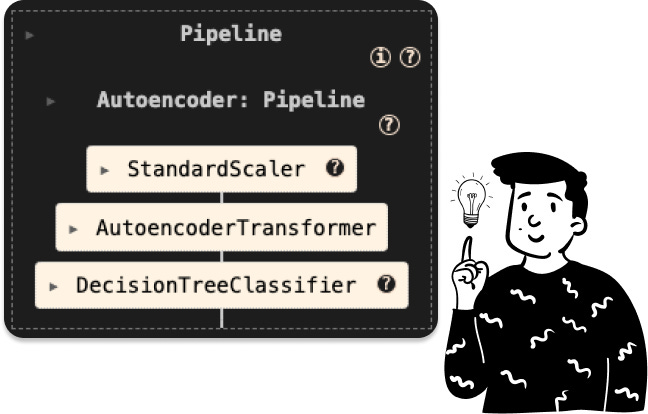
It’s crucial to remember that when we employ the class AutoencoderTransformer, we must specify the output dimension. By default, I set it to 5 (since it matches the size of the LDA). However, in the notebook, I use 35 because I intend to compare it to PCA to determine the most effective pre-processing technique.
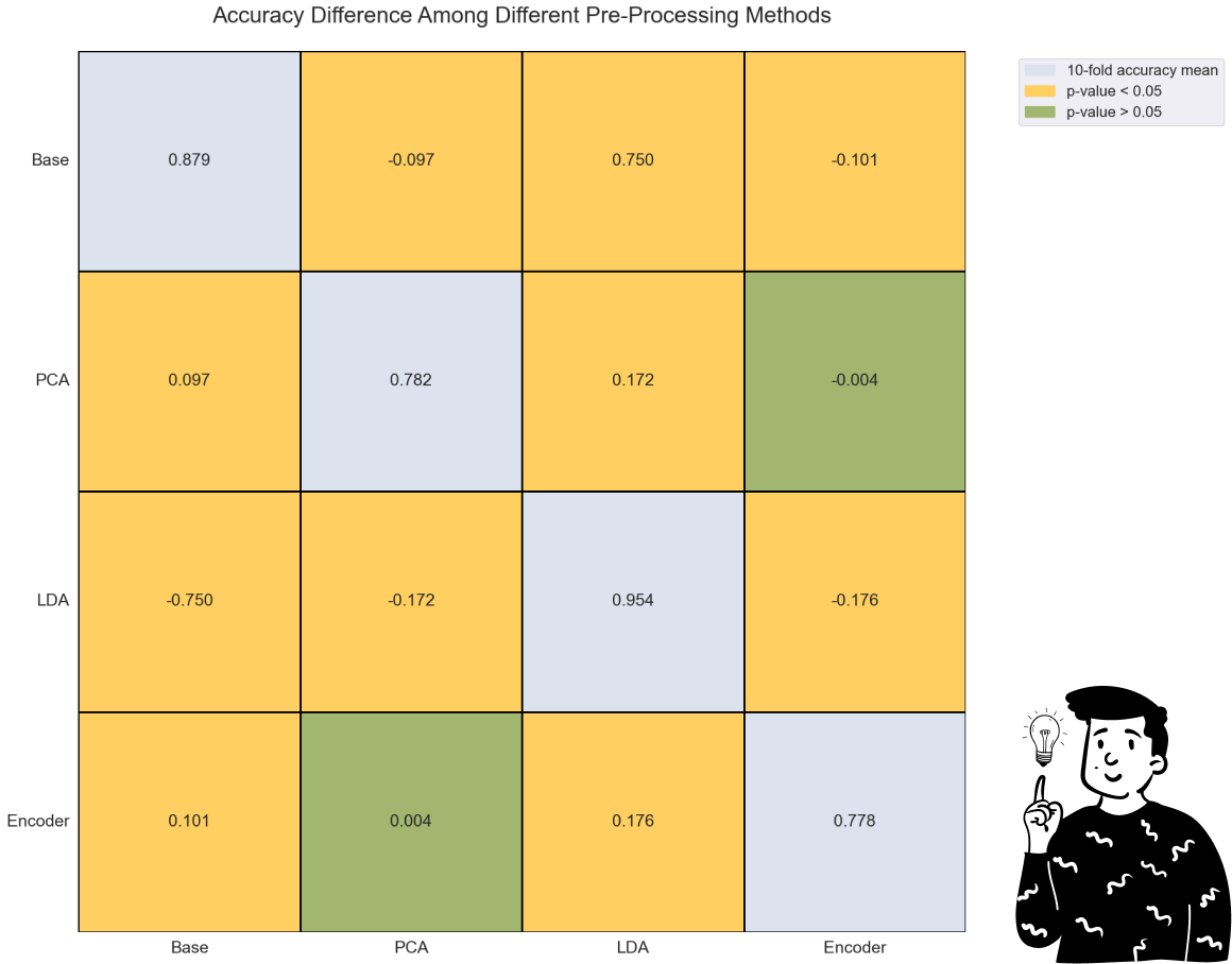
Results
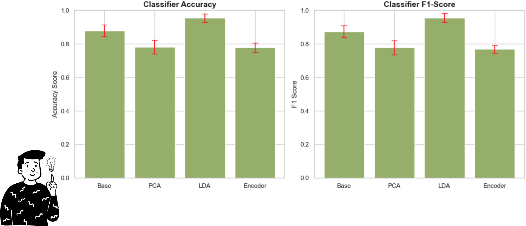
By looking at the plot above, we can clearly see that the LDA performs very well compared to any other pre-processing method. Indeed, even making an ANOVA model with the Bonferroni adjustment, the only comparison that is not significant is the one between the PCA and the Encoder (p>0.833).
Another important result is that both the Accuracy and the F1 score produce the exact same conclusion, so it is interesting to note that the LDA as a pre-processing technique might increase the performance of the Decision tree.
Thanks for your time, if you have any questions be free to ask me, and if you want to run the code by yourself just click here.