LDA in Machine Learning: A Tool for Classification and Feature Extraction

A comprehensive breakdown of Linear and Quadratic Discriminant Analysis, their assumptions, and their practical applications.

Last week, we focused on the first of the two most popular Machine Learning algorithms that make the Bayes Classifier feasible. If you want to understand why we can’t directly use Bayes’ theorem to derive the posterior for a classification problem, I suggest checking out the post I published on

AI Disruption

.

In today’s episode we’ll focus on Discriminant Analysis. Specifically, we’ll cover:

• What Discriminant Analysis is

• The differences between Linear and Quadratic Discriminant Analysis

• Its main assumptions

• Its limitations

What Discriminant Analysis is

Beyond the more common neural networks and advanced algorithms like Gradient Boosting, many classification problems can be effectively tackled by simpler yet powerful methods—Discriminant Analysis is one of them.

There are several ways to interpret and use Discriminant Analysis. In this post we’ll explore two perspectives: the first highlights its role in approximating Bayes’ theorem, while the second presents it as a dimensionality reduction tool. In both cases the assumptions and limitations remain the same; the difference lies in how we derive the method.

How It Makes Bayes’ Theorem Feasible

The core idea behind Bayes’ theorem is to derive a posterior probability (or distribution) for a specific variable given the behavior of other related variables. The formula to compute this probability is as follows:

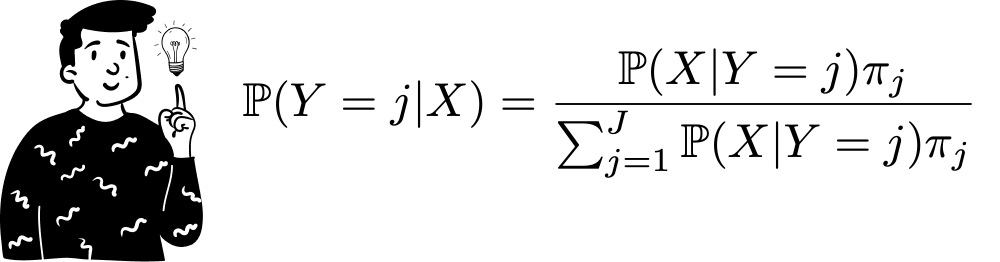
From the previous episode we know that the challenge lies in computing the numerator, while the denominator can be omitted since it acts as a normalizing factor. Here, the algorithm simplifies the numerator to make computation feasible, even with multiple predictors (X).

To achieve this we assume that each predictor follows a normal distribution with a specific mean and variance. This allows us to express the multivariate likelihood as a multivariate Gaussian distribution, varying across each class of the target variable Y. Consequently, computing the numerator reduces to a straightforward multiplication of the likelihood and the associated prior distribution.

At first glance using a multivariate Gaussian as the likelihood function may not seem to resolve any issues. However, looking at its general formula, we understand why it works:

The formula depends on just two parameters, while all other elements are fixed:

• The mean vector of the predictors µ

• The variance-covariance matrix of the predictors Σ

Thus, the algorithm only needs to compute one matrix and one vector to derive the likelihood for each class j-th of the target Y.

Quadratic Discriminant Analysis

In practice, the variance-covariance matrix isn’t always computed for each class. Different Discriminant Analysis techniques handle this differently. Quadratic Discriminant Analysis (QDA) computes a separate variance-covariance matrix for each class, leading to posterior distributions of varying sizes and shapes.

Conversely, if we assume a shared variance-covariance matrix across all classes, the likelihoods will differ only in their means. This results in Gaussian distributions of identical shape but centered at different locations. Since this approach reduces computational complexity and produces linear decision boundaries, it is called Linear Discriminant Analysis (LDA).

Classification

Once we derive the posterior distributions using LDA or QDA, we can determine where a given observation falls in the space. Based on its position, we calculate the relative likelihoods for each class. The predicted class corresponds to the distribution with the highest posterior probability.

LDA as a Dimensionality Reduction Tool

An alternative way to view LDA is as a dimensionality reduction tool that generates latent variables, which best separate the target classes linearly. This interpretation draws a strong parallel with Principal Component Analysis (PCA). Despite their similarities LDA differs in that it requires labeled training data.

In this post I won’t delve deeply into the mathematical details of PCA or LDA. If you’re interested I highly recommend checking out Stanford’s blog post on the topic.

Instead, I want to focus on what these latent variables represent and why they are useful for defining an optimal subspace in which to project observations for better class separation.

2-Class Problem

Let’s assume we are classifying observations into two categories. In this case we aim to combine all available predictors into a new set of variables that can be represented in a lower-dimensional space, where class separation is achieved using linear decision boundaries. In a 2D space, this boundary is a line; in a 3D space, it’s a plane, and so on.

To grasp this concept imagine trying to define the best latent variables for a dataset that appears as follows in a scatterplot:

As you can see no single line can perfectly (or even approximately) separate the two classes.

To address this, we apply the same assumption as before: each predictor follows a Gaussian distribution, conditional on the target class. Consequently the latent variables are also multivariate Gaussian-distributed. When projected onto their new coordinates, the data points remain normally distributed.

To visualize the points we typically use two latent variables. Generally the number of latent variables chosen is smaller than the number of original variables, with the selection based on explained variance. However, in this case, if we retain both latent variables, the resulting plot appears as follows:

Here, the dataset remains the same, but viewed from a different perspective—essentially, it has been projected onto a new subspace. Additionally, the algorithm identifies the optimal linear separator (represented by the dashed line) that maximizes class separation. This line corresponds to the decision boundary where the probability of Y=1 belonging to class exceeds that of Y=0 .

Assumptions

Unfortunately LDA is not always applicable. As you may have noticed, both examples involved categorical target variables. Indeed LDA is not suitable for predicting continuous outcomes—it only supports classification tasks. The reason is intuitive: LDA relies on estimating the variance-covariance matrix of predictors conditioned on the target variable. If the target were continuous, the number of classes would be infinite, making the multivariate function computationally intractable.

Another key assumption concerns the predictors, which must be continuous. The reasons for this constraint are:

• The normal distribution applies only to continuous variables.

• The latent variables are linear combinations of the predictors, and linear combinations inherently require continuous inputs.

I hope you enjoyed this post! If you did, please consider subscribing. See you next week!