


This is a two-part post. The first part, which will be published on AI Disruption, provides an in-depth look at the Bayesian classifier and why it is theoretically the best classifier among all. I highly recommend checking it out for a deeper understanding. Here, I will give a brief introduction to ensure you can follow along with this topic before reading the other post.
A Quick Recap of the Bayes Classifier
In Machine Learning the goal of any classifier is to minimize a metric that quantifies classification errors. The most commonly used metric is the expected classification error rate, which helps us understand how often a model misclassifies observations on average.
From machine learning theory, it can be proven that the best possible classifier—even outperforming the most advanced neural networks—is the Bayes classifier, which classifies observations using posterior probabilities.

In this scenario the unknown parameter we seek to determine is whether or not our target variable belongs to a specific class (e.g., the j-th class).

When multiple predictor variables are involved computing the numerator of Bayes' formula is highly complex. This is because we lack a likelihood function that explicitly defines how all predictors are distributed given the target class. Even for computers, computing such a multivariate function is extremely tedious!
To tackle this problem data science has developed alternative approaches, leading to the creation of several machine learning algorithms. Among them two of the most effective are Naive Bayes and Discriminant Analysis.
In this post, we’ll explore:
What Naive Bayes is
Its main assumptions
How it works with quantitative and qualitative predictors
Its limitations
In the next post, we’ll cover:
What Discriminant Analysis is
Its main assumptions
The differences between Linear and Quadratic Discriminant Analysis
Its limitations
So, let’s get started.
Naive Bayes
As mentioned earlier, the main challenge with Bayes’ theorem when multiple predictors are involved is deriving the associated likelihood. To simplify this both Naive Bayes and Discriminant Analysis make assumptions about the distribution of individual variables. Specifically, Naive Bayes assumes that all predictor variables are independent given the target class.
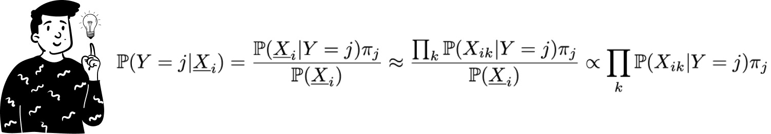
When two variables are independent their joint distribution is simply the product of their marginal distributions. However, note that this assumption does not need to hold universally—only within each target class. This means that for a given class Y = j the conditional likelihood of predictors X and Z can be written as the product of their univariate likelihoods:

Thanks to this property we can compute the posterior probability of the target by multiplying the prior probability of the target class by the product of the univariate likelihoods.
To simplify calculations even further, Naive Bayes ignores the denominator in Bayes’ formula. This exclusion does not significantly impact the classification result, as we only need relative probabilities. This means that Naive Bayes computes each posterior probability as:
Handling Different Types of Variables
To better understand how this algorithm works let's consider an example. Suppose we have a dataset and we want to determine whether a person is a tax evader.

Here, our target variable Y is Evader (Yes/No). The first step is to calculate the prior probabilities of the target:
P(Evader = Yes) = 3/10
P(Evader = No) = 7/10
These probabilities act as weights in the model, indicating how rare or common an event is.
Qualitative variables
Suppose we use Marital Status as a qualitative predictor. To estimate its likelihood Naive Bayes typically applies a multinomial approximation, which involves constructing a histogram of observed frequencies within each target class. This approach allows us to determine the probability of each category appearing within a specific target class based on observed data. By segmenting the observations into different categories, we can better estimate the likelihood of an observation belonging to a certain class.
To illustrate we create two histograms: one for instances where Evader = No and another for instances where Evader = Yes. These histograms show how frequently each marital status appears within each class, forming the basis for our probability estimates. This method provides a straightforward way to model categorical data, making it easier to compute posterior probabilities for classification tasks.

One issue with this approach is that some categories may have zero observations for a particular class. Since the final posterior probability is the product of the univariate likelihoods, having even one likelihood equal to zero nullifies the entire posterior probability. To prevent this we apply the Laplace correction, which adds a small constant to all frequency counts to ensure no probability is exactly zero.
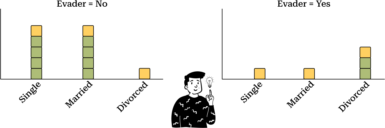
For example, after applying Laplace correction, we get:
P(Single | Evader = Yes) = 5/11
P(Married | Evader = No) = 1/5
Quantitative variables
For continuous variables like Taxable Income, we cannot use simple frequency histograms to estimate probabilities. Instead we must assume a probability distribution. A common choice is the Gaussian distribution. Given this assumption we estimate the mean and standard deviation for each class:
Mean(Taxable Income | Evader = Yes) = 157,500
Std(Taxable Income | Evader = Yes) =88,388
Mean(Taxable Income | Evader = No) = 90,625
Std(Taxable Income | Evader = No) =23,212
However, another approach is the kernel density estimation method. It provides a way to estimate the probability density function of the variable without assuming a specific distributional form. This method is particularly useful when the data does not appear to follow a normal distribution. By applying a smoothing function, such as a Gaussian kernel, KDE produces a continuous curve that approximates the true distribution of the data. Unlike histograms, which depend on bin widths and can be rough approximations, KDE provides a smoother representation of the probability distribution.
This means that the two distributions will be:

To derive the likelihood for a specific value the procedure is straightforward: you simply locate the point on the X-axis and then determine the corresponding points on the Y-axis, one for each distribution. The values obtained will be used to compute the Naive Bayes classifier.
Now, suppose we want to classify a subject who is married and has a Taxable Income of $100,000. To do this, we find the associated probabilities for each target class and then factor in the prior probability of the discriminant class.
On the other hand, the probability that the subject is not an evader, given the same predictor values, is:
Since the posterior probability of not being an evader is higher than that of being one, the Naive Bayes classifier will classify the subject as a non-evader.
Limitations of Naive Bayes
While Naive Bayes is simple and efficient, its strong assumptions lead to several limitations:
Zero-Probability Problem
First of all, as seen in the example above, we must keep in mind that factorization can cause significant issues when dealing with rare events. Specifically, when a qualitative predictor has no occurrences for a particular target class, the derived posterior probability will be null. As a result, the contribution of other variables will vanish due to the factorization.
One solution, as mentioned, is to apply the Laplace correction. However, when dealing with very few observations, even adding an artificial observation that shouldn’t be there can distort the entire analysis.
Small Likelihood
If you examine the derived posterior probabilities you’ll notice that both values are very small. This is due to the likelihood associated with the Taxable Income variable, which is very low. The issue of a vanishing posterior can arise even without a completely null value—if at least one likelihood is extremely small, the entire posterior will also be small.
Context problem
Multiplication follows the commutative property, meaning that the order in which we multiply the different likelihoods does not affect the result. However, in many domains, such as sentiment analysis, word order is just as important as the words themselves. This is a major limitation of Naive Bayes in such contexts.
If you’d like to learn more about this issue or Naive Bayes in general, I highly recommend watching this video:
Collinearity
The last and most important drawback is that Naive Bayes suffers from multicollinearity. This means that if two or more predictors are strongly correlated, the results become inconsistent and distorted.
The root of this issue lies in the key assumption of Naive Bayes: that all predictors are mutually uncorrelated, given the target class. When this assumption is violated, we end up calculating the multivariate likelihood using an incorrect formula, leading to erroneous posterior estimates.
Conclusion

Hope you enjoyed today’s episode! In the next one, we’ll cover Discriminant Analysis. In the meantime, you can check out the post about the Bayes Classifier on AI Disruption.