


In this brief series of posts about Bayesian statistics, I will cover some fundamental aspects I studied at university. This series will be divided into three posts, each continuing from the previous one.
The posts are divided into:
The Bayes theorem and the different kinds of distributions
How the decision-making process works (focusing on AI)
The Markov chain and the Monte Carlo algorithm

The Bayes theorem
All of Bayesian theory revolves around a simple formula formulated almost three hundred years ago by the eponymous Thomas Bayes. Symbolically, it is expressed as:
In words, this means that given two events (event A and event E), the probability of observing A conditioned on E is proportional to the probability of observing E conditioned on A.
The Dice Problem
At first glance, this concept might be difficult to digest. It becomes clearer when we define the term conditioned, which appears on both sides of the equation and is represented by the symbol "|".
The conditional probability P(A∣E) can be thought of as the probability of event A happening, but only in the context where event E has already occurred. Essentially, it focuses on the portion of A's probability that manifests only when E is true.
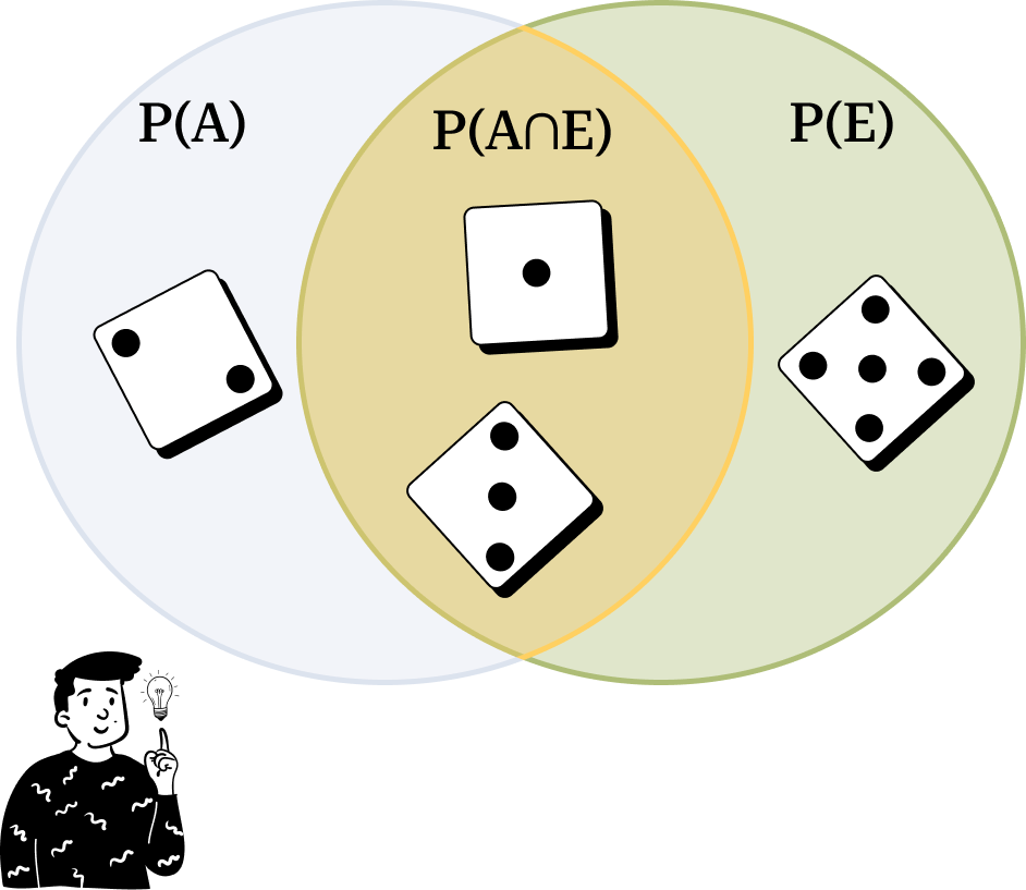
For example, consider this question: What is the probability of rolling a dice and obtaining a value less than 4, knowing that the value is odd?
This question involves two events:
Event A: Finding a number less than 4.
Event E: Knowing the number is odd.
o calculate P(A∣E), we consider the elements in each set. By examining the dice outcomes:
Region A contains the values {1,2,3}, so it has 3 elements.
Region E contains {1,3,5}, so it also has 3 elements.
The region where A and E overlap contains {1,3}, which has 2 elements.
The probability P(A∣E) is therefore the fraction of elements in both regions (2) over the elements in E (3):
Now that this concept is more clear we can finally give a better definition of the Bayes theorem.
Conceptual Approach
In practice, the Bayes theorem updates our understanding of an event based on new information. For instance, calculating the probability of finding a number less than 4 without any additional information involves more uncertainty than when we know the number is odd.
Imagine two people ask you to bet $10 on event A. Would you prefer to bet with someone who tells you the number rolled is odd or with someone who provides no information at all?
AI Approach
The dice example is just one of many scenarios illustrating Bayes' theorem. This formula allows us to update our knowledge of an event by observing its manifestations. Consider your Instagram feed: Meta’s algorithm (like those of other social networks) predicts your likelihood of engaging with specific posts. This probability must be dynamic—every time you like a post, the algorithm updates itself to reduce uncertainty about your preferences.

A similar approach is used in AlphaChip, the AI agent developed by DeepMind to design chips faster and smarter.

In my previous post, I introduced Markov chains, which are rooted in Bayesian statistics. By definition, Markov chains use only the information from the previous step to make decisions at the current step. Doesn't this sound quite similar to the dice example?
From Probability to Function
In practice, the Bayes theorem operates using functions. These functions serve as both inputs and outputs of the theorem:
Prior function (π(θ)): Describes the behavior of the parameter we aim to update, without any observations. For example, this could be the probability distribution an LLM uses to predict the first word of a sentence before receiving any input.
Conditional function (f(x∣θ), or Likelihood): Represents the probability of observing data used to update the prior distribution.
The result of applying the Bayes theorem is the posterior function (π(θ∣x)), which contains all the updated information about the parameter of interest.
In the original theorem, there’s a denominator that represents the distribution of x, independent of θ. Since this is often difficult to derive, we simplify by focusing on the numerator. The posterior distribution becomes proportional to the product of the prior distribution and the likelihood.
Posterior Distribution
Understanding probability distributions can be challenging, especially in the context of AI. However, every time you query an LLM, each word in its response is governed by a probability distribution. This can be viewed as a posterior distribution, where the parameter θ represents the underlying structure of the language model, including its learned weights and parameters. In essence, the posterior distribution reflects the model’s updated belief about the next word, given the sequence of words you’ve already provided.

Exercise
Before concluding, here's an exercise from my course. At first glance, it seems straightforward, but solving it requires a solid grasp of the concepts discussed above:
Suppose a guilty person fails a lie detector test with a probability of 0.95, while an innocent person passes the test with a probability of 0.90. During a bank robbery, the police detain six people, including two actual robbers. One suspect is chosen at random for a lie detector test. If the lie detector indicates the person is guilty, what is the probability they really are guilty?
To resolve this problem, we use the Bayes theorem. Let’s define the events:
A: The person is guilty.
E: The lie detector test indicates guilt.
From the problem, we know:
Using Bayes' theorem:
Substituting the values:
The probability that the person is guilty, given that the lie detector indicates guilt, is approximately 82.6%.
Hope you have enjoyed this first post about Bayesian statistics, in the next weeks I will roll out next episodes.
(Probably if you click on my account you can already see the next episode)