

Fact-checking AI, episode 4 - Pre-processing the query with the semantics chunking

Since the last episode of this series, many things have changed on my blog. If this is the first post you’re reading about this series, let me introduce you to the project I’m currently working on.
Resume:
My friend and I are eager to learn more about the world of large language models (LLMs) and some of the principal techniques behind them. For this reason, we decided to start a project focused on fact-checking AI. Our goal is to build an AI agent that can analyze a chunk of text—such as a tweet—and determine whether it contains false information. In the previous episodes, we outlined at a high level what the model needs to do with the user-provided text and how to retrieve sources to verify the information.

Why focusing on the query
Over the past month Daniel and I have had many discussions about the key aspects of our idea that need improvement. After several meetings we decided to start with the RAG system. In a previous episode I discussed different types of RAG systems and how to choose one. Specifically, we believe that the retrieval process strongly depends on how we pre-process the query. The generation process can also be improved by providing structured examples to train the model to systematically produce formatted outputs.
Pre-processing
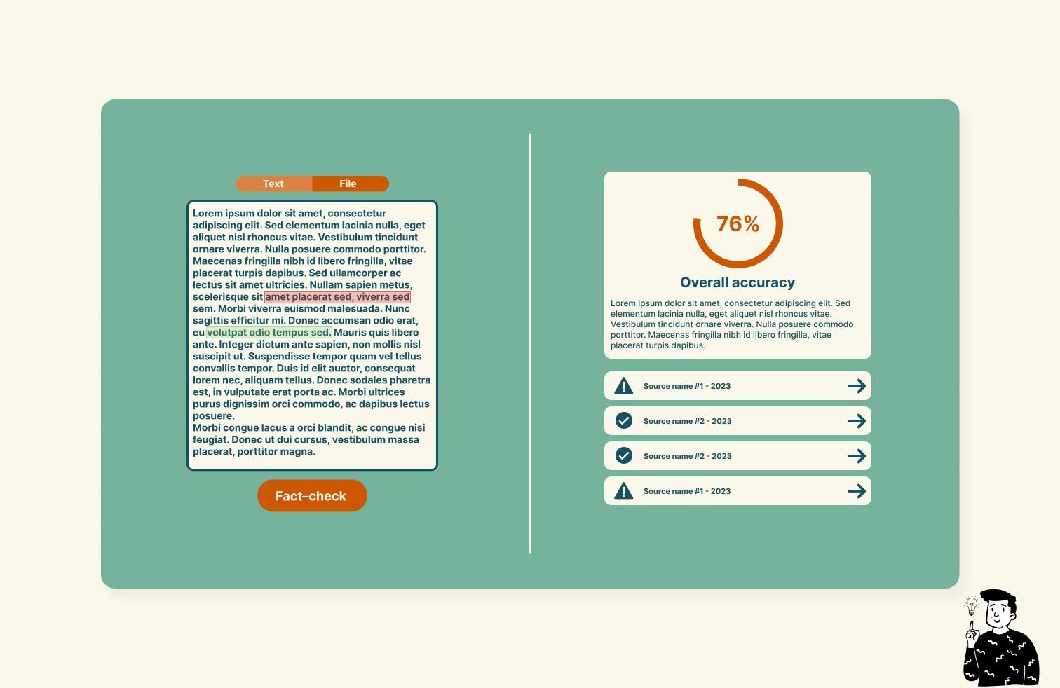
When we talk about pre-processing the user-provided text, the term can mean many things. To clarify our goal is to simplify the project as much as possible: we take a text input and have the AI fact-check different phrases by providing both a source and a “credibility score.”
The first challenge arises: how can the AI identify where one phrase ends and another begins?
When we look at our X (Twitter) or Substack feeds, posts often contain multiple phrases that may not be semantically related. For example consider this tweet:
The earth is flat and the WW2 occurred between the 1939 and the 1945.
Here the two statements are unrelated. The first is false, while the second is true. In such cases the AI must define the boundaries between phrases before analyzing each one to determine its truthfulness.
Semantics chunking
Separating text into meaningful phrases is a complex process, with many methods available (each with pros and cons). The simplest approach is to split the text after a fixed number of characters, letters, or tokens—similar to how we chunk source articles.
However in this case precision is key. Thus, we opted for a more sophisticated approach: semantic chunking.
Semantic chunking divides text into meaningful sections by analyzing relationships between parts of the text. It involves calculating similarities between chunks, using vector representations of sentences or words. If two text segments are similar they are grouped into semantically coherent chunks. To detect sentence boundaries we calculate the Euclidean distance between embeddings of consecutive sentences. A large distance jump signals that the sentences are semantically unrelated, marking the end of a chunk.
Defining the parameters
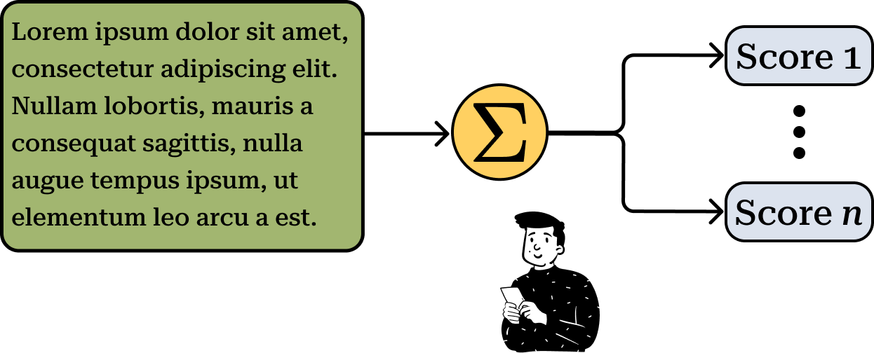
Graphically the semantics chunking is a kind of sliding windows that is placed above the text, at each window’s position the vector generated will have different coordinates:
To visualize this I created an animation showing the “sliding window” in action.
To implement this, we need to define two elements:
The span of the window
The threshold that determines when a phrase ends
Both parameters were determined by analyzing the dataset of news articles we collected in Episode 2.

Daniel wrote a script to calculate the Euclidean distance between sentences in a text using a sliding window. The script tests spans of 2, 4, 6, and 8 phrases. While I won’t delve into the code I’ll highlight a clever approach we used to define a phrase.
Sentence Splitting Without LLM
There are many different kinds of small models that can be deployed to divide a long text into its words. For example, one of the most popular libraries available is spaCy, a NLP model compatible with many national languages (Source).
However for this script we decided not to use another LLM. Instead we aimed to find a smarter solution that doesn’t rely on any neural network or similar technology:
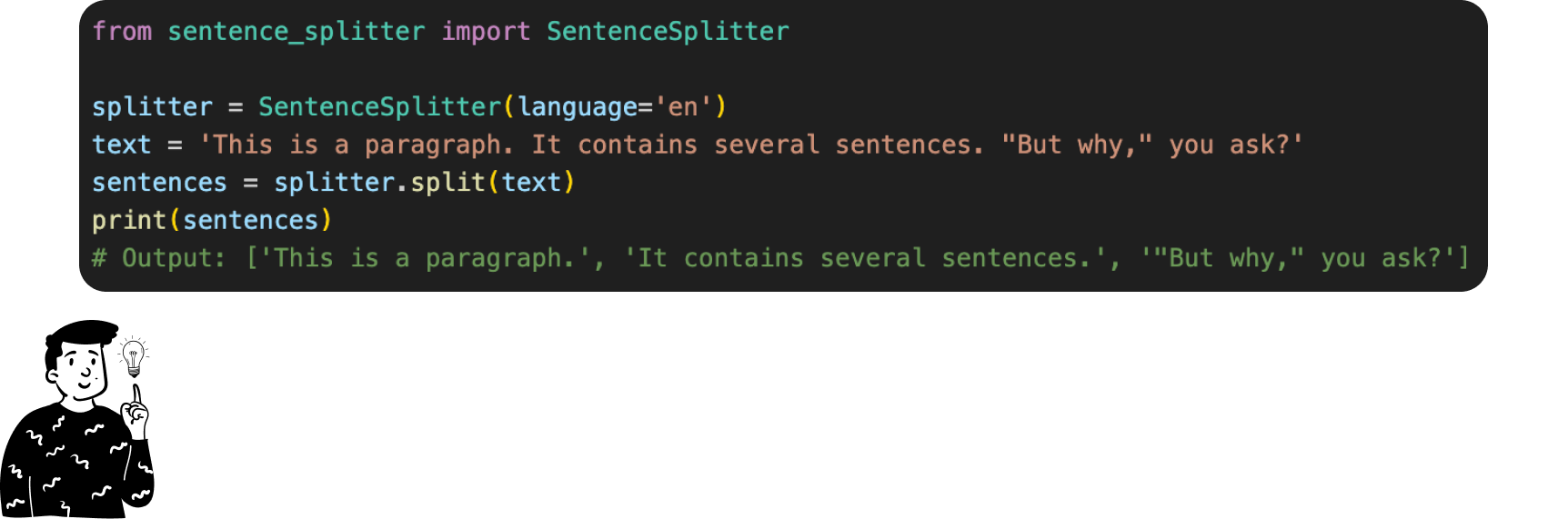
The sentence-splitter uses rules and heuristics inspired by the Europarl corpus1, a dataset widely used for language processing. It works by:
Detecting Sentence-End Punctuation: It identifies sentence boundaries using standard punctuation marks like periods, question marks , and exclamation points.
Leveraging Non-Breaking Prefixes: To avoid splitting prematurely (e.g., after abbreviations like "Dr." or "etc."), it uses a list of non-breaking prefixes derived from the Europarl corpus.
Checking Capitalization: After a potential sentence-ending punctuation, it checks if the next word starts with a capital letter, a common signal for a new sentence.
These rules, based on linguistic patterns in the Europarl corpus, allow us to handle complex sentence structures effectively across multiple languages.
Embedding analysis
After applying the sliding window to embed sentences I analyzed the optimal span and threshold distance to distinguish one topic from another.
Daniel’s script generated data for four window sizes (2, 4, 6, 8), stored in JSON files. Each entry contained:
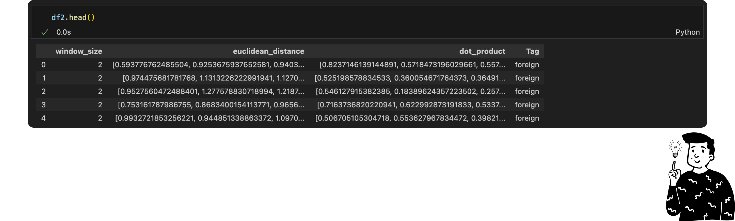
window_size: The number of phrases in the sliding window.euclidean_distance: The distance between consecutive embeddings.dot_product: Similarity metric using dot products.Tag: The article's category.
Interestingly, increasing the span reduced the number of observations. At first, I suspected a bug in the script, but the Pandas documentation clarified that empty rows are excluded from sample counts. This indicates that larger spans are more likely to encounter texts too short to process.
By increasing the span Pandas recognizes fewer observations. At first glance I thought there was an issue with the script used to embed text. However after reviewing the Pandas documentation I discovered that empty rows are not counted in the total sample size. This clarified that the larger the span the higher the likelihood of encountering text too short to be processed.
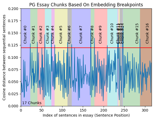
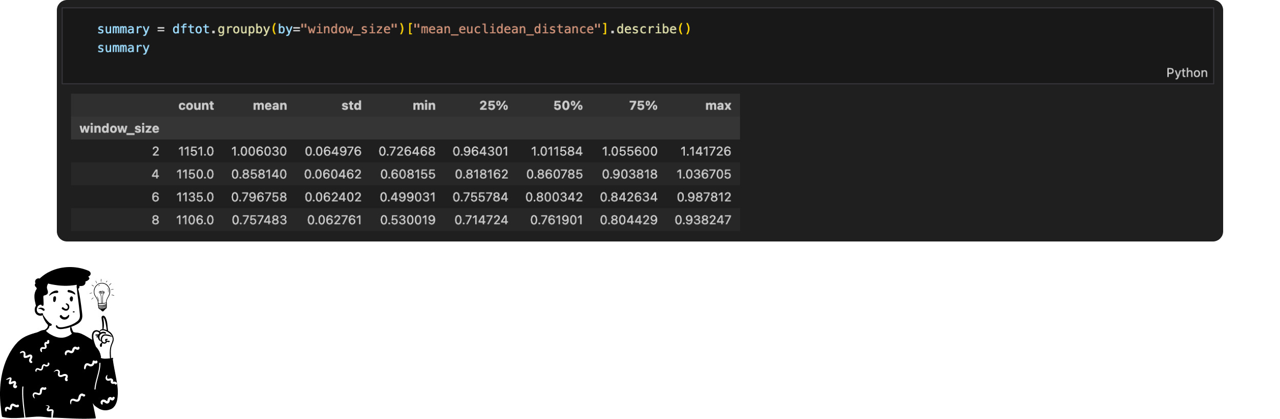
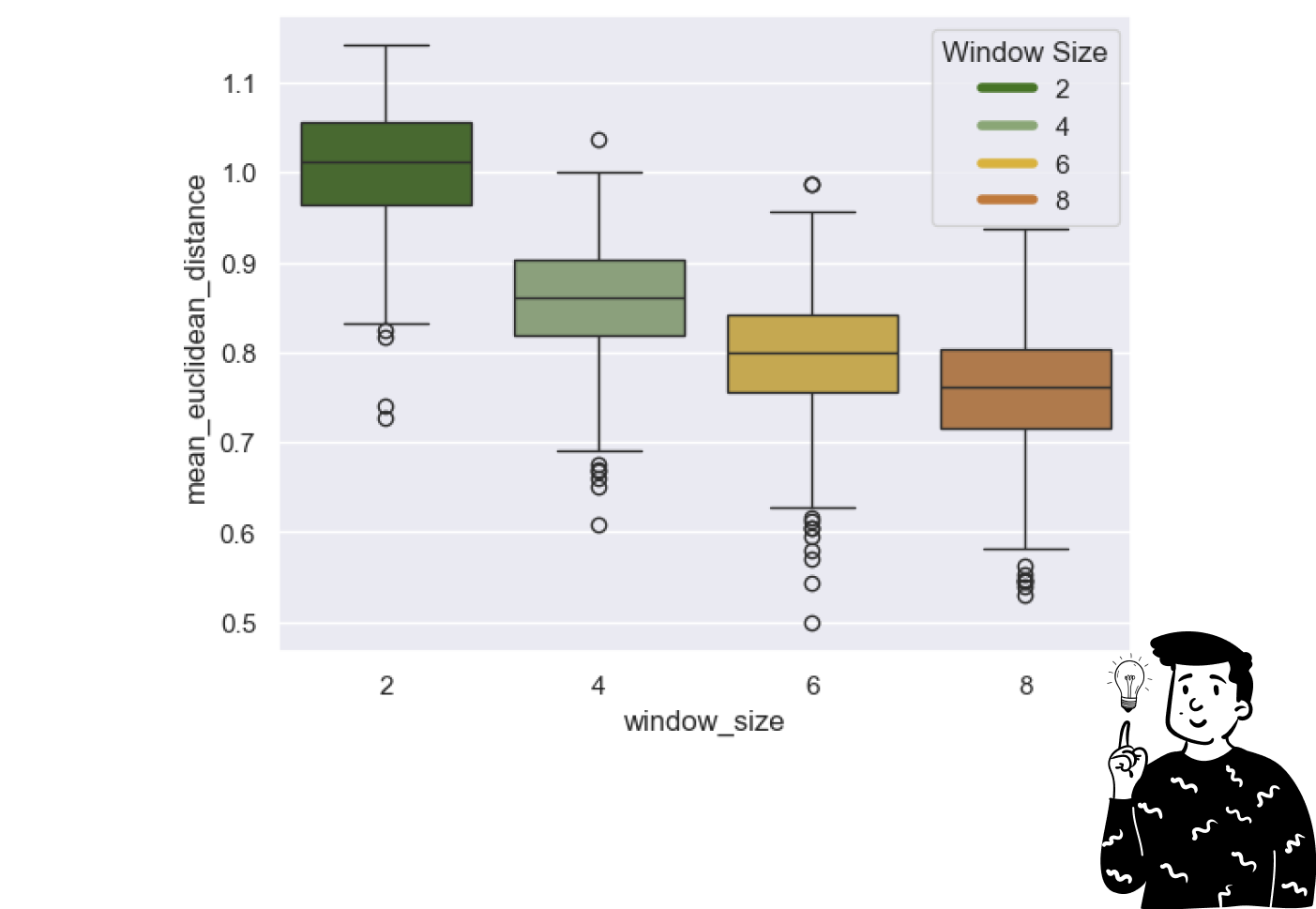
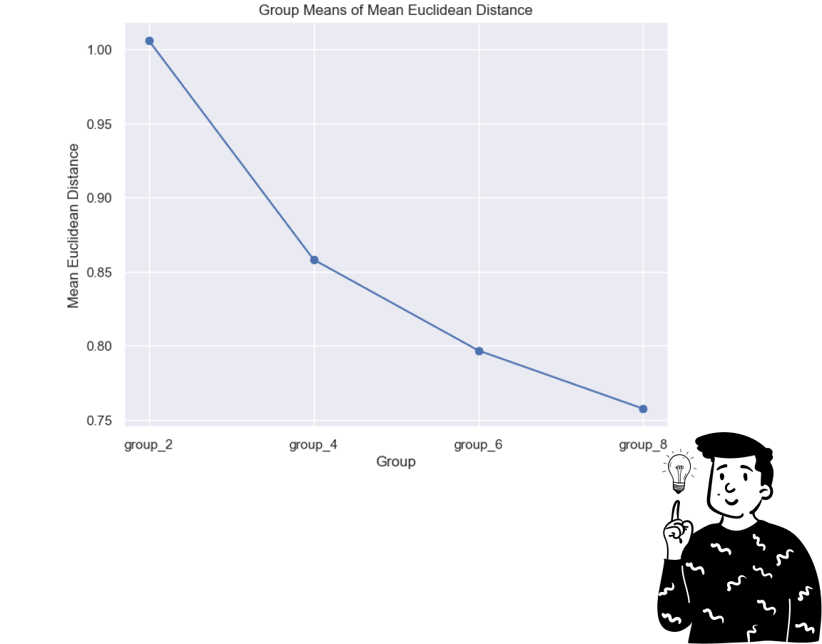
Despite this inconvenience in the code above I first calculated the sample mean for each list of the window_size. Using these means I calculated the overall sample mean for each span. Under the "mean" column, you can observe that, on average, the distance between consecutive phrases decreases as the span increases. Graphically this looks like:
In statistics a common method for determining whether group means differ significantly is the ANOVA test. While I won’t delve into the theory here—it deserves a post of its own—here’s a simplified explanation: imagine the means I calculated represent sample estimates. In reality there could be many possible values that were missed due to randomness or other factors. The ANOVA test evaluates whether the observed differences in the sample are due to random variation or reflect real differences in the population.
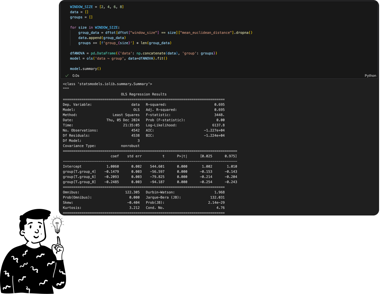
To perform the ANOVA, I used the following code. Personally I prefer using the model instead of the test because it directly provides both the lsmeans and p-values. If you’re unfamiliar with these terms, don’t worry; for now, focus on two important columns:
coef: The first row displays the mean of the first group, while subsequent rows show the difference between the respective group’s mean and the first group’s mean. For example, the lsmean for a span of 4 is calculated as 1.0060−0.14979=0.856211.0060−0.14979=0.85621.P>|t|: This column represents the probability that the difference between group means and the first group is zero. In this case the probability is nearly zero, indicating the difference is statistically significant.
The trend of the lsmeans reflects the mean Euclidean distance. To ensure the robustness of these inferences I verified the assumption of homoscedasticity (equal variance of errors). While I won’t include the full process here, you can find it in the markdown file I published on GitHub. The hypothesis of equal variance was confirmed, ensuring that the inferences are correct.
I also conducted t-tests between the different groups, using Bonferroni’s correction for multiple comparisons. All groups were found to have significantly different means.
Conclusion
Based on these statistical tests we decided to use a span of 8 phrases for semantic chunking. This decision was based on two key factors:
Vector Distance: The shorter the distance between vectors, the more coherent the text becomes, enabling the model to better understand the provided sentences. According to the lsmeans, the span of 8 phrases produces vectors that are 5.18% closer than those with a span of 6 phrases. This difference is statistically significant.
Phrase Coverage: Only 3.9% of phrases were too short to be processed with a span of 8, which is an acceptable outcome for our project.
The plan is to design an algorithm that defaults to using a span of 8 phrases for semantic splitting. If the text is too short, it will adapt by using spans of 6, 4, or smaller, eventually operating without any span at all.
The threshold distance for differentiating sentences will be calculated as the lsmean plus its standard deviation. For instance, when using a span of 8, the threshold will be:
(Probably if you click on my account you can already see the next episode)